Kernelized Factor Models (Thinking Aloud)
Last update: 15 Jul 2025 22:19First version: 27 March 2024, with a "why think, when you can do the experiment?" update on 31 March
Attention conservation notice: If there's any merit to this, someone else has probably done it already. Indeed, it's very possible that I am channeling stuff I've read but consciously forgotten.
Since I'd just been teaching factor models, a student in advanced data analysis who'd taken machine learning classes featuring kernel machines asked if there was anything like a kernelized factor model. I actually couldn't remember anything that was quite that, but it set me thinking, so I'll just record my thoughts.
The natural way to kernelize a linear model or method is to express everything in terms of inner products, and then replace those inner products with uses of the kernel function. If we think about the model in factor analysis, \( \vec{X} = \mathbf{w} \vec{F} + \epsilon \), we can express that in terms of inner products by saying \( X_i = \vec{w}_i \cdot \vec{F} + \epsilon_i \), \( i \in 1:p \), where \( \vec{w}_i \) is the \( i^{\mathrm{th}} \) row of the loadings matrix \( \mathbf{w} \). The natural kernelization of this would be \( X_i = K(\vec{u}_i, \vec{F}) + \epsilon_i \), \( i \in 1:p \). So it's be parameterized by \( p \) \( q \)-dimensional vectors \( \vec{u}_1, \vec{u}_2, \ldots \vec{u}_p \), and by the noise variances.
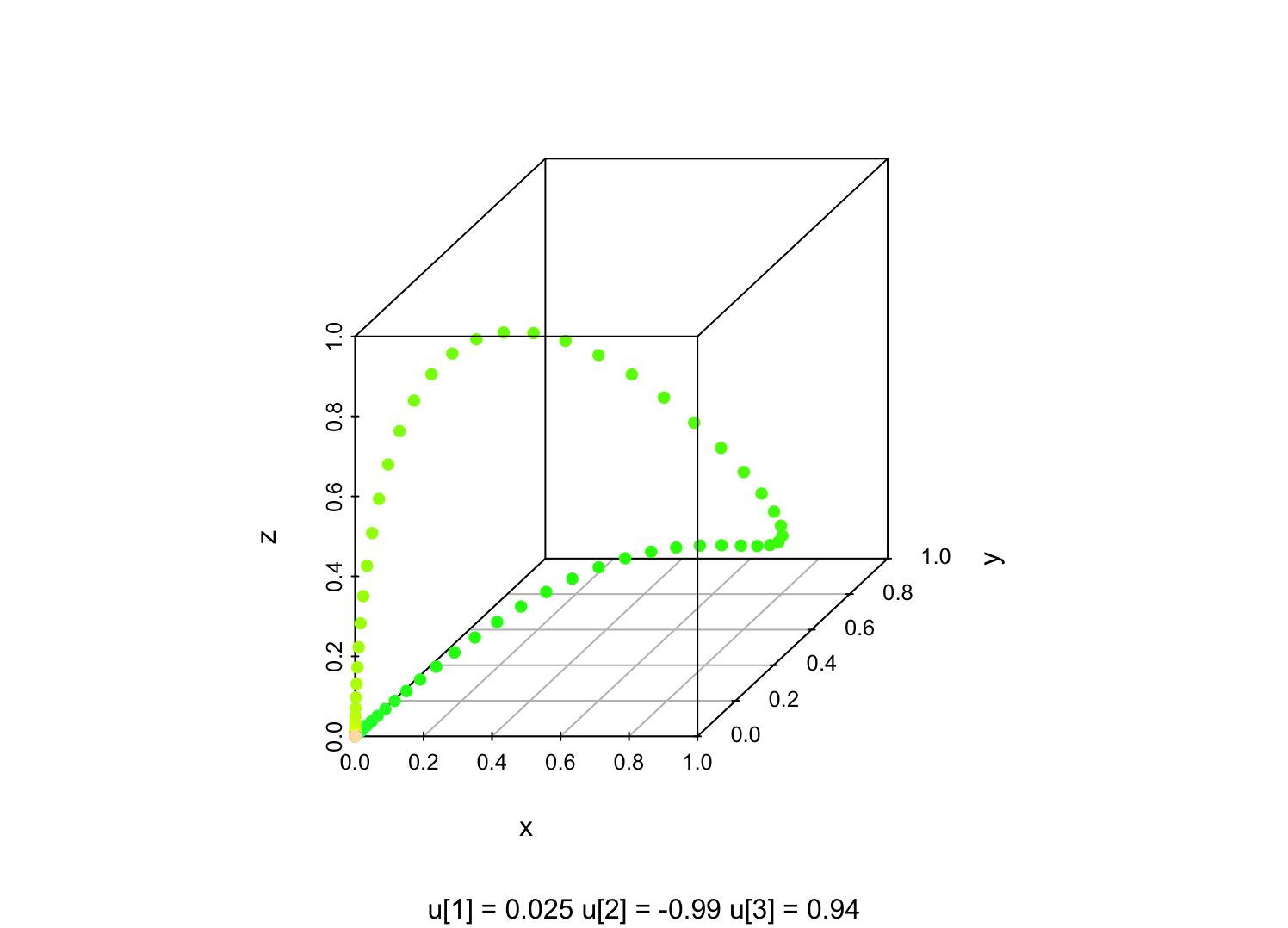
For ordinary factor models, if we hold the loading matrix \( \mathbf{w} \) fixed and let the factor score vector \( \vec{F} \) vary, \( \mathbf{w}\vec{F} \) will trace out a \( q \)-dimensional linear subspace of \( \mathbb{R}^p \), and then the noise \( \epsilon \) perturbs us off that. In the kernelized version of that, holding the \( \vec{u}_i \) fixed and letting \( \vec{F} \) vary, we'll trace out a \( q \)-dimensional curved manifold in \( \mathbb{R}^p \). For instance, with a Gaussian kernel, \( K(u,v) = e^{(u-v)^2} \), if I set \( q=1 \), \( p=3 \), and pick three random numbers for \( u_1, u_2, u_3 \), sweeping \( F \) from \( -10 \) to \( 10 \) gives me a picture like this (color-coding the value of \( F \)):
library(scatterplot3d)

# Hard-codes $p=3$, $q=1$ but OK for now
x.from.f <- function(f, loadings=c(u1, u2, u3)) {
  x1 <- exp(-(loadings[1]-f)^2)
  x2 <- exp(-(loadings[2]-f)^2)
  x3 <- exp(-(loadings[3]-f)^2)
  return(data.frame(x=x1, y=x2, z=x3))
}

u1 <- rnorm(1)
u2 <- rnorm(1)
u3 <- rnorm(1)

x <- x.from.f(seq(from=-10, to=10, length.out=200))

# Plot it, color-coding $F$ (since I've generated in order of increasing $F$)
scatterplot3d(x, color=topo.colors(200), pch=16,
              sub=paste(expression(u[1]), "=", signif(u1,2),
                        expression(u[2]), "=", signif(u2,2),
                        expression(u[3]), "=", signif(u3,2)))

Fixing the kernel, but varying the vectors \( \vec{u}_i \), gives \( pq \) adjustable parameters which can change either the manifold, or the distribution on the manifold. In a similar way, in a linear factor model, the loading matrix \( \mathbf{w} \) gives \( pq \) adjustable parameters to change the linear subspace and/or the distribution on it. If we multiply \( \mathbf{w} \) by a scalar, we don't change the linear subspace in which \( \mathbf{w}\vec{F} \) lives, but we do change the distribution on that subspace. If we insert an orthogonal matrix and its inverse between the factors and the loadings, $(\mathbf{w}\mathbf{o}) (\mathbf{o}^T \vec{F})$, we change neither the subspace nor the distribution on it, we just change the coordinate system we use on the subspace.
Queries:
- For what classes of kernels is there an analog of the rotation problem in linear factor models? (Presumably lots?)
- Can we say anything about the dimension of the family of manifolds we get by varying the \( \vec{u}_i \), either in general, or for interesting classes of kernels?
I feel like the answer here has to involve the answer to the previous question. The space of orthogonal $q\times q$ matrices has dimension $\frac{q(q-1)}{2}$, so the dimension of the maximal identifiable parameter of a linear factor model is at most $\frac{q}{2} (2p - q + 1)$. But since I am asking specifically about the dimension of the family of manifolds, parameter changes which only alter the distribution on the manifold do not count here. - If we use a polynomial kernel, is the manifold an algebraic variety?
Assuming a fixed kernel function, you could try to estimate such a model by alternating minimization:
- Taking the current guess at all the latent factor scores as fixed, find the \( \vec{u}_i \in \mathbb{R}^q \) which minimizes the mean squared error between the actual values of \( X_i \) and \( K(\vec{u}_i, \vec{F}) \). Do this in parallel for each of the \( p \) observables \( X_i \).
- Taking the current guess at the loading vectors \( \vec{u}_i \) as fixed, find the factor scores which best match the observables (in parallel across units).
- We probably want an explicit intercept vector, rather than centering everything, so another minimization step...
# Calculate expected positions given loadings and factor scores matrix
# Inputs:
  # array of factor scores (f), n*q dimensional
  # array of loadings (u), p*q dimensional
  # vector of intercepts (u), p dimensional
# Outputs: n*p dimensional matrix of numerical values
# Presumes:
  # both u and f have q columns
  # alpha has p columns
  # Gaussian kernel of fixed bandwidth
  # TODO: flexibility for bandwidth and/or kernel
ekfm <- function(f, u, alpha=0) {
   q <- ncol(f)
   stopifnot(ncol(u) == q)
   p <- nrow(u)
   if (length(alpha)==1) { alpha <- rep(alpha, times=p) }
   stopifnot(length(alpha)==p)
   # Do one coordinate of one point...
   ekfm.ij <- function(u.vec, f.vec) { exp(-sum((u.vec-f.vec)^2)) }
   # Do all coordinates of one point
  # generate all the coordinates of one data point
    # Include the intercept here
    # TODO: Nicer way to vectorize?
  ekfm.i <- function(f.vec) { alpha + apply(u, 1, ekfm.ij, f.vec=f.vec) }
  # generate a big array of coordinates
    # turn on the side so it has as many rows as f did
  ekfm <- t(apply(f, 1, ekfm.i))
  return(ekfm)
}
# Draw from a kernelized factor model
# Inputs:
  # number of points to draw (n)
  # function to generate random factor scores (rfactor)
  # array of u vectors (u)
  # vector of "uniquenesses"/noise variances (psi)
  # vector intercepts (alpha, default 0)
# Output: an array of observable vectors
# Presumes:
  # rfactor is a no-argument function generating q-dimensional vectors
  # u is a p*q array
  # psi is a p dimensional vector
  # alpha is a p-dimensional vector
rkfm <- function(n, rfactor, u, psi, alpha=0) {
  # Dimension of the latent-factor space
  q <- ncol(u)
  # Dimension of the observables
  p <- nrow(u)
  # Sanity-check: one noise variance per observable
  stopifnot(p==length(psi))
  # Sanity-check: unless we are giving the same intercept (usually 0!) for each
  # coordinate, should have one intercept per observable
  if (length(alpha)==1) { alpha <- rep(alpha, times=p) }
  stopifnot(p==length(alpha))
  # Make an array of factor scores
    # replicate() returns 1 column per replication, but we want a row per
    # simulated data point so transpose, UNLESS rfactor() returns a scalar
  f <- replicate(n, rfactor())
  if (is.null(dim(f))) {
    f <- matrix(f, ncol=1)
  } else {
    f <- t(f)
  }
  # Calculate the expected coordinates
  expected.observables <- ekfm(f, u, alpha)
  # make some noise
  epsilon <- matrix(rnorm(n=n*p, mean=0,
                          sd=rep(sqrt(psi), times=n)),
                     nrow=n, byrow=TRUE)
  # add the noise to the expected-value part and return
  return(expected.observables + epsilon)
}
# Estimate a kernelized factor model by alternating least squares
# Inputs:
  # data matrix (x)
  # number of factors (q)
  # initial guess at factor scores (initial.scores)
  # initial guess at the loadings
  # initial guess at the intercept
  # numerical tolerance for optimization (tol)
  # maximum number of iterations (itermax)
kfm.als <- function(x, q, initial.scores=NULL,
                    initial.loadings=NULL,
                    initial.intercepts=c(0,0,0),
                    tol=1e-6, itermax=200) {
   # Initialize factor scores using PCA, just to have something fast (if bad)
   if (is.null(initial.scores) || is.null(initial.loadings) || is.null(initial.intercepts)) {
     x.pca <- prcomp(x, retx=TRUE)
     if (is.null(initial.scores)) {
       initial.scores <- x.pca$x[, 1:q]
       if (q==1) {
         initial.scores <- matrix(initial.scores, ncol=1)
       }
     }
     if (is.null(initial.loadings)) {
       initial.loadings <- x.pca[, 1:q]
       if (q==1) {
         initial.loadings <- matrix(initial.loadings, ncol=1)
       }
     }
     if (is.null(initial.intercepts)) {
        initial.intercepts <- x.pca
     }
   }
   new.scores <- initial.scores
   new.loadings <- initial.loadings
   new.intercepts <- initial.intercepts
   l2.prediction.change <- Inf
   iter <- 1
   # define the objective function
   l2.error <- function(f,u,alpha) { sum((x - ekfm(f, u, alpha))^2) }
   # define the three objective functions...
     # optim() wants the optimizand to be the first argument to the function
     # optim() also insists that the argument be a vector...
   l2.error.scores <- function(f) {
      f <- matrix(f, ncol=q)
      return(l2.error(f, current.loadings, current.intercepts))
   }
   l2.error.loadings <- function(u) {
     u <- matrix(u, ncol=q)
     return(l2.error(current.scores, u, current.intercepts))
   }
   l2.error.intercepts <- function(alpha) {
     return(l2.error(current.scores, current.loadings, alpha))
   }
   # store current predictions for observables
   new.preds <- ekfm(f=new.scores, u=new.loadings,
                     alpha=new.intercepts)
   while ((l2.prediction.change > tol) & (iter <= itermax)) {
      # update everything
      preds <- new.preds
      current.loadings <- new.loadings
      current.scores <- new.scores
      current.intercepts <- new.intercepts
      # minimize loadings over fixed factor scores, intercept
      new.loadings <- optim(par=current.loadings, fn=l2.error.loadings)
      # Reshape to matrix because optim flattens everything to vectors
      new.loadings <- matrix(new.loadings, ncol=q)
      current.loadings <- new.loadings
      # minimize factor scores over fixed loadings, intercept
      new.scores <- optim(par=current.scores, fn=l2.error.scores)
      # Reshape to matrix
      new.scores <- matrix(new.scores, ncol=q)
      # minimize intercept over fixed loadings, factor scores
      new.intercept <- optim(par=current.intercepts, fn=l2.error.intercepts)
        # No reshaping necessary since alpha is a vector
      # calculate new predictions
      new.preds <- ekfm(f=new.scores, u=new.loadings, alpha=new.intercepts)
      # calculate squared change in predictions
      l2.prediction.change <- sum((new.preds-preds)^2)
      # increment iterations
      iter <- iter+1
   }
   return(list(scores=new.scores,
               loadings=new.loadings,
               intercepts=new.intercepts,
               iter=iter,
               final.pred.change=l2.prediction.change))
}
z <- rkfm(n=100,
          rfactor=function(){rnorm(1)},
          u=matrix(c(0.025, -0.99, 0.94), ncol=1),
          psi=c(0.001, 0.001, 0.001))
z.s3d <- scatterplot3d(z, pch=16)
z.s3d(ekfm(f=matrix(seq(from=-10, to=10, length.out=200), ncol=1),
                    u=matrix(c(0.025, -0.99, 0.94), ncol=1)),
               col="green", type="l", lty="solid")
z.fit <- kfm.als(z, q=1, initial.intercepts=c(0,0,0))
z.s3d(ekfm(f=z.fit, u=z.fit), col="blue", pch=16)
z.s3d(ekfm(f=matrix(seq(from=-10, to=10, length.out=200), ncol=1),
                    u=z.fit),
               col="blue", type="l", lty="dashed")

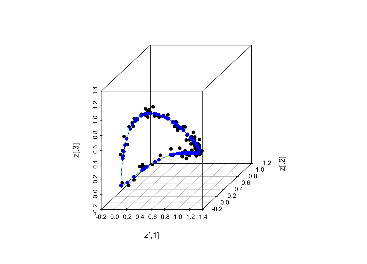
Green line = underlying manifold (same "loadings" as in previous figure); black dots = random sample of points on manifold plus perturbations off it (noise variance = 0.001 for each observable coordinate); blue dots = reconstructed positions from the iterative, alternating-minimization procedure; dashed blue line = reconstructed manifold.
TODO:
-
Try out the iterative procedure. ("Why think, when you can do the experiment?", as my mother used to say.)It worked, at least in the demo above! - Can any parts of the iterative procedure be done in closed form, or do I need to brute-force optimize at each step? (The demo above took 4.5 minutes on my 2017-vintage Mac laptop with $n=100$...)
Partial answer, 5 April 2024: Well, the intercepts can be found in closed form! (At least with this least-squares objective.) \( \alpha_i = \overline{X}_i - \frac{1}{n}\sum_{j=1}^{n}{K(\vec{u}_i, \vec{F}_j)} \), i.e., the intercept makes the sample mean and the predicted mean line up, as usual. I should try to carve out an hour to do some math for the other parts of the procedure, though. - Literature search (ask: A.R., A.L., L.W., K.R.).
- See also:
- Manifold Learning
- Have skimmed:
- Darryl Charles and Colin Fyfe, "Kernel factor analysis with Varimax rotation", International Joint Conference on Neural Networks 6 [IJCNN 2000], pp. 381--386 [This just does an analogy to kernel PCA, focused on estimating factor scores. It doesn't really consider a generative model or its parameters. However, there may be a generative model implicit in their estimation procedure, which I should think through carefully. --- This paper has only been cited 6 times, per Google Scholar, but appears to have evoked the sincerest form of flattery.]