Laplace Approximation

Last update: 07 Dec 2024 23:54
First version: 8 March 2024

Attention conservation notice: Lightly-dusted-off teaching notes, plus references.

a.k.a. "Laplace's method", "Laplace's principle", etc. In short: The surprising effectiveness, when faced with an integral of the form $\int{e^{nf(x)} dx}$, of doing a Taylor approximation inside the exponent...

The Basics
More dimensions
Priors and expectations
- Some finger-exercises on Bayesian convergence
- Expectations and large deviations

The Basics

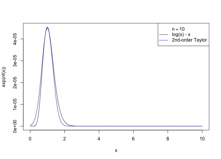
We want to integrate $\int{e^{nf(x)} dx}$ for large $n$. (Using $n$ here is suggestive of a count, like sample size or number of molecules, but that's not really important.) Let's say that $f$ has a maximum at $x^*$. Now $e^{nf(x^*)}$ is, literally, exponentially larger than $e^{nf(x)}$ for any $x \neq x^*$. So it's not crazy to think that the integral is going to end up being dominated by contributions from $x^*$, and maybe points nearby. (On the other hand, it's not obvious either --- there are a lot more points which are far from the maximum, so maybe their integrated contributions dominate.)

Let's start by pretending that $x$ is one-dimensional (we'll lift this in a few paragraphs), and that there's a well-behaved interior maximum at $x^*$. That means that $f^{\prime}(x^*) = 0$ and $f^{\prime\prime}(x^*) < 0$. (This is important and I will not get rid of it.) For later convenience, define $s=1/|f^{\prime\prime}(x^*)|$. Taylor-expand $f$ to second order around the maximum: \[ f(x) \approx f(x^*) + \frac{1}{2}(x-x^*)^2 f^{\prime\prime}(x^*) \] Now stick this in the exponent and integrate: \begin{eqnarray} \int{e^{nf(x)} dx} & \approx & \int{e^{nf(x^*)} e^{\frac{1}{2}(x-x^*)^2 f^{\prime\prime}(x^*)} dx}\\ & = & e^{nf(x^*)} \int{e^{-n\frac{(x - x^*)^2}{2s}}dx}\\ & = & e^{nf(x^*)} \int{e^{-\frac{(x - x^*)^2}{2(s/n)}} dx} \end{eqnarray} I have manipulated things this way because I remember, from baby prob., the form of a Gaussian probability density, and the fact that it integrates to 1: \[ \int{\frac{1}{\sqrt{2\pi \sigma^2}}e^{-(u-\mu)^2/2\sigma^2} du} = 1 \] (Now why that is true, I honestly can never remember, and I have to re-imprint the argument on my memory whenever I need to teach that part of baby prob. [1]) Hence \[ \int{e^{-(u-\mu)^2/2\sigma^2} du} = \sqrt{2\pi\sigma^2} \] Apply that here: $x^*$ takes the role of $\mu$, $s/n$ the role of $\sigma^2$, hence \begin{eqnarray} \int{e^{nf(x)} dx} & \approx & e^{nf(x^*)} \int{e^{-\frac{(x - x^*)^2}{2(s/n)}} dx}\\ & = & e^{nf(x^*)} \sqrt{2\pi s/n}\\ & = & e^{nf(x^*)} \sqrt{\frac{2\pi}{n |f^{\prime\prime}(x^*)|}} \end{eqnarray}

Exponential decay instead of exponential growth

If we had wanted to do $\int{e^{-nf(x)} dx}$, then we would go through an entirely parallel derivation, only with $x^*$ being the location of the minimum of $f$, and $s=f^{\prime\prime}(x^*)$ (because the 2nd derivative will be positive at a minimum). The conclusion is entirely parallel: \[ \int{e^{-nf(x)} dx} \approx e^{-nf(x^*)} \sqrt{\frac{2\pi}{n |f^{\prime\prime}(x^*)|}} \]

On the log scale

Suppose we just care about the exponential growth rate for the integral of $e^{nf(x)}$. (Or decay rate of the integral of $e^{-nf(x)}$; as just explained, it all works the same.) That, we have just seen, is \begin{eqnarray} \lim_{n\rightarrow\infty}{\frac{1}{n}\int{e^{n f(x)} dx}} & \approx & \lim{\frac{1}{n} \left( nf(x^*) - \frac{1}{2}\log{n} - \frac{1}{2}\log{|f^{\prime\prime}(x^*)} + \frac{1}{2}\log{2\pi} \right)}\\ & = & f(x^*) - \frac{1}{2}\frac{\log{n}}{n} + \frac{\log{|f^{\prime\prime}(x^*)} + \log{2\pi}}{2n} \end{eqnarray} That is, the growth rate is just given by the maximum value of $f(x^*)$ of $f$. Everything else is $o(1)$ in $n$: in more detail, an $O(\frac{\log{n}}{n})$ contribution that only depends on the dimension, and an $O(1/n)$ contribution from the second derivative.

Approximation error

Having co-written a whole paper which largely turned on being careful about the approximation error of this method, I should feel like expounding that here, but honestly I do not. See the references.

A traditional application: Stirling's formula

Here is a cute (and traditional) illustration of what we have just done. Like many people raised as physicist, I have essentially one tool for dealing with combinatorics problems, which is Stirling's formula for factorials, \[ \log{n!} \approx n\log{n} - n \] This is, believe it or not, actually an instance of Laplace approximation. There are three steps to getting here:

Re-write $n!$ as an integral, using the gamma function.
Re-write the integrand into the form $e^{nf(x)}$.
Turn the Laplace-approximation crank and then take the log.

Re-write $n!$ as an integral: At some point, one of the Ancestors --- I have no idea if it was Stirling or Euler or someone else --- noticed the following: \[ \int_{0}^{\infty}{x^n e^{-x} dx} = n \int_{0}^{\infty}{x^{n-1} e^{-x} dx} ~ (*) \] (I will explain how to prove this in a minute.) They were then inspired to draw a connection to the factorial function, since $n! = n (n-1)!$. Happily, if we keep recursing, we get \[ \int_{0}^{\infty}{x^n e^{-x} dx} = n (n-1) (n-2) \ldots (2) (1) \int_{0}^{\infty}{e^{-x} dx} \] and even I can evaluate that last integral and see that it $=1$, so \[ n! = \int_{0}^{\infty}{x^n e^{-x} dx} \]

As for showing (*), use the integration trick with the impenetrable name of "integration by parts", which is really just the product rule for derivatives: \begin{eqnarray} d(uv) & = & u dv + v du\\ \int_{a}^{b}{d(uv)} & = & \left. uv \right|_{a}^{b} = \int_{a}^{b}{u dv} + \int_{a}^{b}{v du}\\ \therefore \int_{a}^{b}{u dv} & = & \left. uv \right|_{a}^{b} - \int_{a}^{b}{v du} \end{eqnarray} Setting $u=x^n$ and $v=-e^{-x}$, so that $ dv=e^{-x} dx $, gives \begin{eqnarray} \int_0^{\infty}{x^n e^{-x} dx} & = & \left.-x^n e^{-x}\right|_0^{\infty} - \int_0^{\infty}{\left(-e^{-x}\right) n x^{n-1} dx} & = & 0-0 + n\int_0^{\infty}{x^{n-1} e^{-x} dx}\\ & = & n\int_{0}^{\infty}{x^{n-1} e^{-x} dx} \end{eqnarray} as claimed.

($\int{x^n e^{-x} dx}$ shows up often enough that it gets a name; we call it the "gamma function", and write it with an upper-case $\Gamma$. It is almost the continuous generalization of the factorial function. However, the standard definition is that $\Gamma(n) \equiv \int_{0}^{\infty}{x^{n-1} e^{-x} dx}$, so that what we have shown is $n! = \Gamma(n+1)$, whereas $n! = \Gamma(n)$ would look much nicer. The annoying off-by-one in the definition of the gamma function does simplify some other formulas, however, which will not concern us here.)

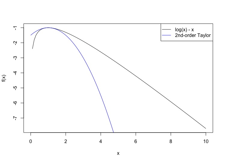
Re-write the integrand in the form $e^{nf(x)}$: The integrand is \[ x^n e^{-x} = e^{n\log{x} - x} \] Define $u=x/n$, so $\log{x} = \log{n} + \log{u}$, and $ dx = n du $. \begin{eqnarray} n\log{x} - x & = & n(\log{n} + \log{u}) - nu\\ & = & n\log{n} + n(\log{u} - u)\\ n! & = & \int_{0}^{\infty}{e^{n\log{x} -x} dx}\\ & = & \int_{0}^{\infty}{e^{n\log{n}} e^{n(\log{u} - u)} n du}\\ & = & e^{n\log{n}} n \int_{0}^{\infty}{e^{n(\log{u} - u)} du} \end{eqnarray} that is, $f(u) =\log{u} - u$.

Turn the Laplace-approximation crank: $f^{\prime}(u) = 1/u - 1$ and $f^{\prime\prime}(u) =-u^{-2}$, so $u^* = 1$, $f(u^*) = - 1$, $f^{\prime\prime\prime}(u^*)=-1$. Plugging in, \begin{eqnarray} \int_{0}^{\infty}{e^{n(\log{u} - u)} du} & \approx & e^{-n} \sqrt{\frac{2\pi}{n}}\\ n! & \approx & e^{n\log{n}} n e^{-n}\sqrt{\frac{2\pi}{n}}\\ & = & e^{n\log{n} - n} \sqrt{2\pi n}\\ \log{n!} & \approx & n\log{n} - n + \frac{1}{2}\log{n} + \frac{1}{2}\log{(2\pi)} \end{eqnarray}

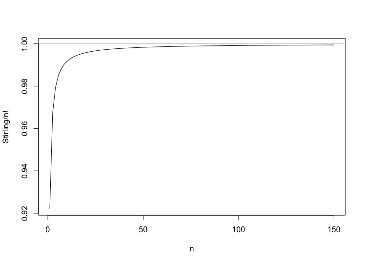
The approximation is startlingly good even for small $n$ (which is part of why generations of teachers have used this example). The first five factorials are of course 1, 2, 6, 24, 120. The approximations, using this form of Stirling-via-Laplace, are $0.922$, $1.92$, $5.84$, $23.5$ and $118$. A plot of the ratio is as boring as anyone could hope:

More dimensions

If $x$ is $d$-dimensional, then we replace the second derivative with the Hessian matrix of second partials: \[ f(x) \approx f(x^*) + \frac{1}{2} (x-x^*) \cdot (\nabla \nabla f(x^*)) (x-x^*) \] Turning the Gaussian-integral crank in the exact same way, \[ \int{e^{nf(x)} dx} \approx e^{n f(x^*)} \sqrt{\frac{(2\pi)^d}{n |\nabla\nabla f(x^*)|}} \]

Priors and expectations

Suppose the integral is of the form \[ \int{e^{nf(x)} p(x) dx} \] for some non-negative function $p$. This will arise if $p(x)$ is a probability density function and we are taking the expectation of $e^{nf(x)}$. An especially important instance of that is when we are doing Bayesian statistics, with $p(x)$ being the prior, and $f(x)$ the average log-likelihood per observation.

The obvious approach is to take a log and work $p(x)$ into the exponent: \[ \int{e^{nf(x)} p(x) dx} = \int{e^{n(f(x) + \frac{1}{n}\log{p(x)})} dx} \] Now, all of the previous argument rested on $f(x)$ not changing as $n\rightarrow\infty$, but since we obviously left mathematical rigor far behind long ago, we might as well just apply the machinery to $ g_n(x) \equiv f(x) + \frac{1}{n}\log{p(x)} $.

The thing to notice, though, is that $ g_n \rightarrow f $ as $n$ grows. If we are interested in the location of the optimum, well, Taylor-expand $g^{\prime}_n(x)$ around the $x^*$ which optimizes $f$ alone, set it to zero at $\tilde{x}_n$, and solve: \begin{eqnarray} g^{\prime}_n(x) & \approx & \frac{1}{n}\frac{p^{\prime}(x^*)}{p(x^*)} +(x-x^*)\left(f^{\prime\prime}(x^*) + \frac{1}{n}\frac{p^{\prime\prime}(x^*)}{p(x^*)}\right)\\ 0 & = & \frac{1}{n}\frac{p^{\prime}(x^*)}{p(x^*)} + (\tilde{x}_n - x^*))\left(f^{\prime\prime}(x^*) + \frac{1}{n}\frac{p^{\prime\prime}(x^*)}{p(x^*)}\right)\\ \tilde{x}_n & = & x^* - \frac{1}{n}\frac{p^{\prime}(x^*)}{p(x^*)} \frac{1}{f^{\prime\prime}(x^*) + \frac{1}{n}\frac{p^{\prime\prime}(x^*)}{p(x^*)}}\\ & \approx & x^* - \frac{1}{n}\frac{p^{\prime}(x^*)}{p(x^*) f^{\prime\prime}(x^*)}\left(1 - \frac{1}{n}\frac{p^{\prime\prime}(x^*)}{p(x^*) f^{\prime\prime}(x^*)}\right) \end{eqnarray} That is, the optimum of $ g_n $ is located at the optimum $x^*$ of $f$, plus corrections that are $O(1/n)$ at best. (Of course this presumes that $p(x^*) \neq 0$.)

Since we are interested in large $n$, \[ \int{e^{nf(x)} p(x) dx} \approx p(x^*) e^{nf(x^*)} \sqrt{\frac{2\pi}{n|f^{\prime\prime}(x^*)|}} \] and similarly for the higher-dimensional version.

Now, this is not necessarily the best way of using Laplace's approximation in this situation; whether we get a bigger or smaller approximation error by evaluating everything at the optimum of $f$, or by including the way $p$ shifts the optimum, can be a little delicate. (See Tierney, Kass and Kadane.)

Some finger-exercises on Bayesian convergence

We are estimating a $d$-dimensional parameter $\theta$. The Bayesian agent's prior pdf on the true parameter is $\pi_0(\theta)$. The likelihood of seeing the data $ X_1=x_1, X_2=x_2, \ldots X_n=x_n $ is $ L_n(x_{1:n};\theta) $; because the data are fixed throughout the calculations that follow, I will abbreviate this as just $ L_n(\theta) $. The posterior distribution is \[ \pi_{n}(\theta) = \pi_0(\theta) \frac{L_n(\theta)}{\int{L_n(\theta^{\prime}) \pi_0(\theta^{\prime}) d\theta^{\prime}}} \] (I have my reasons for writing it this way.) Of course this is the same as \[ \pi_n(\theta) = \pi_0(\theta) \frac{e^{-n\Lambda_n(\theta)}}{\int{e^{-n\Lambda_n(\theta^{\prime})} \pi_0(\theta^{\prime}) d\theta^{\prime}}} ~ (**) \] where $\Lambda_n(\theta) = -n^{-1} \log{L_n(\theta)}$ is the average negative log likelihood per observation. I do this, of course, so that the denominator looks more like a Laplace-style integral.

The point which maximizes $\Lambda_n(\theta)$ is of course just the maximum likelihood estimate, $\hat{\theta}_n$. The Hessian at the MLE is often written as $\mathbf{K}_n$. So if we apply Laplace approximation to the denominator, we get \begin{eqnarray} \pi_n(\theta) & \approx & \pi_0(\theta) \frac{e^{-n \Lambda_n(\theta)}}{\pi_0(\hat{\theta}_n) e^{-n\Lambda_n(\hat{\theta}_n)} (2\pi)^{d/2}/\sqrt{n|\mathbf{K}_n|}}\\ & = & \frac{\pi_0(\theta)}{\pi_0(\hat{\theta}_n)}\frac{\sqrt{n|\mathbf{K}_n|}}{(2\pi)^{d/2}}e^{-n(\Lambda_n(\theta) - \Lambda_n(\hat{\theta}_n))} \end{eqnarray} Since we are assuming that $\Lambda_n(\theta)$ behaved well enough around its maximum to make Laplace approximation worth trying in the first place, we can say that \[ \Lambda_n(\theta) \approx \Lambda_n(\hat{\theta}_n)) + \frac{1}{2}(\theta-\hat{\theta}_n) \cdot \mathbf{K}_n (\theta-\hat{\theta}_n) \] and therefore \begin{eqnarray} \pi_n(\theta) & \approx & & = & \frac{\pi_0(\theta)}{\pi_0(\hat{\theta}_n)}\frac{\sqrt{n|\mathbf{K}_n|}}{(2\pi)^{d/2}}e^{-\frac{1}{2}(\theta-\hat{\theta}_n) \cdot n\mathbf{K}_n (\theta-\hat{\theta}_n)} \end{eqnarray} which is to say that we are getting a basically Gaussian posterior pdf, centered at the MLE, with a variance matrix that comes from the Hessian of the log-likelihood. Cleaned up and made more rigorous, this bit of hand-waving becomes the "Bernstein-von Mises theorem", though my understanding is that getting this result is basically why Laplace invented this method of approximation.

Before leaving this topic, I cannot resist one additional step. We know, from information theory that, for a very wide range of processes, when the actual data-generating distribution is $\mu$, \[ \Lambda_n(\theta) \rightarrow h(\mu) + d(\mu\|\theta) \] where $h(\mu) =$ the entropy rate of the data source, and $d(\mu\|\theta)$ is the growth rate of the Kullback-Leibler divergence between the true distribution and the one implied by the Bayesian's model with parameter $\theta$. This is the "generalized asymptotic equipartition property", and the convergence happens almost surely. (If we're only interested in IID data, we can get this just using the ordinary law of large numbers, but with dependence there's more interesting probability.) Let's go back to (**) and apply this, blithely ignoring the difference between $\Lambda_n$ and its deterministic limit: \[ \pi_n(\theta) \approx \pi_0(\theta) \frac{e^{-n d(\mu\|\theta)}}{\pi_0(\theta^*) e^{-nd(\mu\|\theta^*)} (2\pi)^{d/2} / \sqrt{n\mathbf{k}}} \] where $\theta^*$ is the minimizer of $d(\mu\|\theta)$, and $\mathbf{k}$ is the Hessian of $d(\mu\|\theta)$ at $\theta^*$. Let us take logs and divide by $1/n$ to look at the decay rate of the posterior density: \begin{eqnarray} \frac{1}{n}\log{\pi_n(\theta)} & \approx & d(\mu\|\theta^*) - d(\mu\|\theta) + O(n^{-1/2}) \end{eqnarray} In words: the posterior density goes to zero exponentially fast everywhere, except at the parameter value $\theta^*$ which minimizes the divergence between the model and the true distribution. If you want to see that argument cleaned up, I have a paper for you...

Expectations and large deviations

Above, I presented $p(x)$ as an unchanging probability distribution, and $e^{nf(x)}$ as the exponentially growing, or shrinking, quantity which we are trying to average over that distribution. One can however reverse figure and ground here (as it were). There many situations where, for large $n$, the log probability of some configuration $x$ is $\propto -nf(x)$. Many of these situations arise in statistical mechanics, but you can see how distributions like that will tend to arise whenever we have outcomes involving lots of not-too-dependent, identically-distributed random variables. (See under large deviations.) More specifically, then, the probability density will take the form \[ \frac{e^{-nf(x)}}{\int{e^{-nf(y)} dy}} \] The expectation of some un-changing function $h(x)$ under this distribution will then be \begin{eqnarray} \int{h(x) \frac{e^{-nf(x)}}{\int{e^{-nf(y)} dy}} dx} & = & \frac{\int{h(x) e^{-nf(x)}} dx}{\int{e^{-nf(y)} dy}}\\ & \approx & h(x^*) \end{eqnarray} shamelessly applying Laplace to the numerator and denominator separately and then canceling everything out.

(An interesting mathematical question is to go the other way: if we have a sequence of probability distributions $ P_n $, and, for all well-behaved functions $h$, $\int{h(x) dP_n(x)} \rightarrow h(x^*)$, is it the case that $ P_n $ approaches having the limiting pdf $\propto e^{-nf(x)}$ for some $f$ minimized at $x^*$? The answer is basically yes, but nailing that down requires rather more precision about probability distributions [measures!] and limits than I have been operating with here --- see Dupuis and Ellis.)

: Here is the (highly traditional) story I usually tell my students. Let us agree to call $c=\int_{-\infty}^{\infty}{e^{-x^2/2}dx}$. Now $c^2=\left( \int_{-\infty}^{\infty}{e^{-x^2/2}dx} \right) \left( \int_{-\infty}^{\infty}{e^{-x^2/2}dx} \right) = \int_{-\infty}^{\infty}{\int_{-\infty}^{\infty}{e^{-x^2/2} e^{-y^2/2} dy} dx}$. (If you want to get formal: use Fubini's theorem.) Change to polar coordinates, so $r^2=x^2+y^2$ (that's Pythagoras), $ dx dy = r dr d\theta $, and thus $c^2 = \int_{r=0}^{\infty}{\int_{\theta=0}^{2\pi}{r e^{-r^2/2} dr d\theta}} = 2\pi\int_{r=0}^{\infty}{r e^{-r^2/2} dr}$. One final change of variable: $u\equiv r^2/2$, so $ du = r dr $, and we get $c^2 = 2\pi\int_{u=0}^{\infty}{e^{-u} du} = 2\pi$. This is correct and elementary, but find it a bit unsatisfying. If you did not know, to start with, that the answer involved a square root, why would it occur to you to do a double integral to find the square of a single normalizing constant? ^