Prediction Processes; Markovian (and Conceivably Causal) Representations of Stochastic Processes

16 Apr 2024 13:45

\[ \newcommand{\indep}{\mathrel{\perp\llap{\perp}}} \newcommand{\Prob}[1]{\mathrm{Pr}\left( #1 \right)} \]

This descends from the slides for a talk I've been giving, in some form, since working on the papers that became my dissertation in the late 1990s.

0. "State"

In classical physics or dynamics, the state of a system is the present variable which fixes all future observables. In quantum mechanics, we back away from determinism: the state is the present variable which determines the distribution of observables. We want to find states, in this sense, for classical stochastic processes. So long as we're asking for things, it would be nice if the state space was in some sense as small as possible, and it would be further nice if the states themselves were well-behaved --- say, homogeneous Markov processes, so we don't have to know too much about probability theory.

We'll try to construct such states by constructing predictions.

1. Notation

Upper-case letters are random variables, lower-case their realizations. We'll deal with a stochastic process, $ \ldots, X_{-1}, X_0, X_1, X_2, \ldots $. I'll abbreviate blocks with the notation $ X_{s}^{t} = (X_s, X_{s+1}, \ldots X_{t-1}, X_t) $. The past up to and including $ t $ is $ X^t_{-\infty} $, future is $ X_{t+1}^{\infty} $. For the moment, no assumption of stationarity is needed or desired.

(Discrete time is not strictly necessary, but cuts down on measure theory.)

2. Making a Prediction

We look at $ X^t_{-\infty} $ , and then make a guess about $ X_{t+1}^{\infty} $. The most general guess we can make is a probability distribution over future events, so let's try to do that unless we find our way blocked. (We will find our way open.)

When we make such a guess, we are going to attend to selected aspects of $ X^t_{-\infty} $ (mean, variance, phase of 1st three Fourier modes, ...). This means that our guess is a function, or formally a statistic, of $ X^t_{-\infty} $.

What's a good statistic to use?

3. Predictive Sufficiency

We appeal to information theory, especially the notion of mutual information. For any statistic $ \sigma $, \[ I[X^{\infty}_{t+1};X_{-\infty}^t] \geq I[X^{\infty}_{t+1};\sigma(X_{-\infty}^t)] \] (This is just the "data-processing inequality".) $ \sigma $ is predictively sufficient iff \[ I[X^{\infty}_{t+1};X_{-\infty}^t] = I[X^{\infty}_{t+1};\sigma(X_{-\infty}^t)] \] Sufficient statistics, then, retain all predictive information in the data.

At this point, the only sane response is "so what?", perhaps followed by making up bizarre-looking functionals and defining statistics to be shmufficient if they maximize those functionals. There is however a good reason to care about sufficiency, embodied in a theorem of Blackwell and Girshick: under any loss function, the optimal strategy can be implemented using only knowledge of a sufficient statistic --- the full data are not needed. For reasonable loss functions, the better-known Rao-Blackwell theorem says that strategies which use insufficient statistics can be improved on by ones which use sufficient statistics.

Switching our focus from optimizing prediction to attaining sufficiency means we don't have to worry about particular loss functions.

4. Predictive States

Here's how we can construct such sufficient statistics. (This particular way of doing it follows Crutchfield and Young [1989], with minor modifications.)

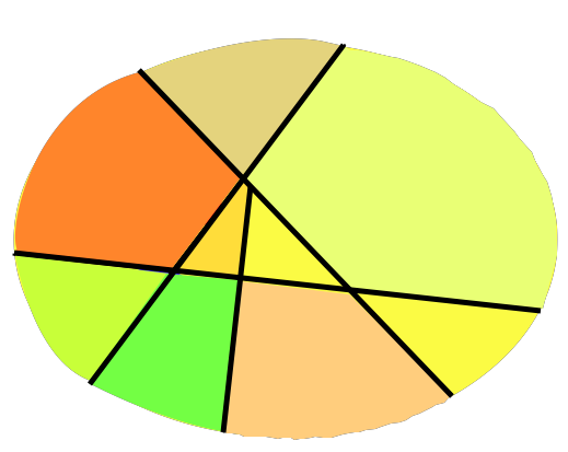
Say that two histories $ u $ and $ v $ are predictively equivalent iff \[ \Prob{X_{t+1}^{\infty}|X_{-\infty}^{t} = u} = \Prob{X_{t+1}^{\infty}|X_{-\infty}^{t} = v} \] That is, two histories are predictively equivalent when they lead to the same distribution over future events.

This is clearly an equivalence relation (it's reflexive, symmetric and transitive), so it divides the space of all histories up into equivalence classes. In the usual symbols, $ [u] $ is the equivalence class containing the particular history $ u $. The statistic of interest, the predictive state, is \[ \epsilon(x^t_{-\infty}) = [x^t_{-\infty}] \] That is, we just map histories to their equivalence classes. Each point in the range of $ \epsilon $ is a state. A state is an equivalence class of histories, and, interchangably, a distribution over future events (of the $ X $ process).

In an IID process, conditioning on the past makes no difference to the future, so every history is equivalent to every other history, and there is only one predictive state. In a periodic process with (minimal) period $ p $, there are $ p $ states, one for each phase. In a Markov process, there is usually a 1-1 correspondence between the states of the chain and the predictive states. (When are they not in correspondence?)

The $ \epsilon $ function induces a new stochastic process, taking values in the predictive-state space, where \[ S_t = \epsilon(X^t_{-\infty}) \]

Set of histories, color-coded by conditional distribution of futures

Partitioning histories into predictive states

5. Optimality Properties

A. Sufficiency

I promised that these would be sufficient statistics for predicting the future from the past. That is, I asserted that \[ I[X^{\infty}_{t+1};X^t_{-\infty}] = I[X^{\infty}_{t+1};\epsilon(X^t_{-\infty})] \] This is true, because \[ \begin{eqnarray*} \Prob{X^{\infty}_{t+1}|S_t = \epsilon(x^t_{-\infty})} & = & \int_{y \in [x^t_{-\infty}]}{\Prob{X^{\infty}_{t+1}|X^t_{-\infty}=y} \Prob{X^t_{-\infty}=y|S_t = \epsilon(x^t_{-\infty})} dy}\\ & = & \Prob{X^{\infty}_{t+1}|X^t_{-\infty}=x^t_{-\infty}} \end{eqnarray*} \]

B. Markov Properties I: Screening-Off

Future observations are independent of the past given the predictive state, \[ X^{\infty}_{t+1} \indep X^{t}_{-\infty} \mid S_{t} \] even if the process is not Markov, \[ \newcommand{\notindep}{\mathrel{\rlap{\ \not}\indep}} X_{t+1} \notindep X^t_{-\infty} \mid X_t ~. \] This is because of sufficiency: \[ \begin{eqnarray*} \Prob{X^{\infty}_{t+1}|X^{t}_{-\infty}=x^t_{-\infty}, S_{t+1} = \epsilon(x^t_{-\infty})} & = & \Prob{X^{\infty}_{t+1}|X^{t}_{-\infty}=x^t_{-\infty}}\\ & = & \Prob{X^{\infty}_{t+1}|S_{t+1} = \epsilon(x^t_{-\infty})} \end{eqnarray*} \]

C. Recursive Updating/Deterministic Transitions

The predictive states themselves have recursive transitions: \[ \epsilon(x^{t+1}_{-\infty}) = T(\epsilon(x^t_{-\infty}), x_{t+1}) \] If all we remember of the history to time $ t $ is the predictive state, we can make optimal predictions for the future from $ t $. We might worry, however, that something which happens at $ t+1 $ might make some previously-irrelevant piece of the past, which we'd forgotten, relevant again. This recursive updating property says we needn't be concerned --- we can always figure out the new predictive state from just the old predictive state and the new observation.

In automata theory, we'd say that the states have "deterministic transitions" because of this property (even though there are probabilities).

(I know I said I'd skip continuous-time complications, but I feel compelled to mention that the analogous property is that, for any $h > 0$, \[ \epsilon(x^{t+h}_{-\infty}) = T(\epsilon(x^t_{-\infty}),x^{t+h}_{t}) \] since there is no "next observation".)

To see where the recursive transitions come from, pick any two equivalent histories $ u \sim v $, any future event $ F $, and any single observation $ a $. Write $ aF $ for the compound event where $ X_{t+1} = a $ and then $ F $ happens starting at time $ t+2 $. Because $ aF $ is a perfectly legitimate future event and $ u \sim v $, \[ \begin{eqnarray*} \Prob{X^{\infty}_{t+1} \in aF|X^t_{-\infty} = u} & = & \Prob{X^{\infty}_{t+1} \in aF|X^t_{-\infty} = v}\\ \Prob{X_{t+1}= a, X^{\infty}_{t+2} \in F|X^t_{-\infty} = u} & = & \Prob{X_{t+1}= a, X^{\infty}_{t+2} \in F|X^t_{-\infty} = v} \end{eqnarray*} \] By by elementary conditional probability, \[ \begin{eqnarray*} \Prob{X^{\infty}_{t+2} \in F|X^{t+1}_{-\infty} = ua}\Prob{X_{t+1}= a|X^t_{-\infty} = u} & = & \Prob{X^{\infty}_{t+2} \in F|X^{t+1}_{-\infty} = va}\Prob{X_{t+1}= a|X^t_{-\infty} = v} \end{eqnarray*} \] Canceling (because $ u \sim v $, \[ \Prob{X^{\infty}_{t+2} \in F|X^{t+1}_{-\infty} = ua} = \Prob{X^{\infty}_{t+2} \in F|X^{t+1}_{-\infty} = va} \] Since the future event $ F $ was arbitrary, we've shown $ ua \sim va $.

(If you know enough to worry about how this might go wrong with infinite sample spaces, continuous time, etc., then you know enough to see how to patch up the proof.)

D. Markov Properties, II: The Predictive States

\[ S_{t+1}^{\infty} \indep S^{t-1}_{-\infty}|S_t \] because \[ S_{t+1}^{\infty} = T(S_t,X_{t}^{\infty}) \] and \[ X_{t}^{\infty} \indep \left\{ X^{t-1}_{-\infty}, S^{t-1}_{-\infty}\right\} | S_t \] One can further show that the transitions are homogeneous, i.e., for any set $ B $ of predictive states, \[ \Prob{S_{t+1} \in B|S_t = s} = \Prob{S_{2} \in B|S_1 = s} \] This is because (by the definition of the predictive states) \[ \Prob{X_{t+1}|S_t=s} = \Prob{X_2|S_1=s} \] and $ S_{t+1} = T(S_t, X_{t+1}) $ (by the recursive-updating property).

E. Minimality

A statistic is necessary if it can be calculated from --- is a function of --- any sufficient statistic. A statistic which is both necessary and sufficient is minimal sufficient. We have seen that $ \epsilon $ is sufficient; it is also easy to see that it is necessary, which, to be precise, means that, for any sufficient statistic $ \eta $, there exists a function $ g $ such that \[ \epsilon(X^{t}_{-\infty}) = g(\eta(X^t_{-\infty})) \] Basically, the reason is that any partition of histories which isn't a refinement of the predictive-state partition has to lose some predictive power.

A non-sufficient partition of histories

Effect of insufficiency on predictive distributions

So there certainly can be statistics which are sufficient and not the predictive states, provided they contain some superfluous detail:

Sufficient, but not minimal, partition of histories

There can also be coarser partitions than those of the predictive states, but they cannot be sufficient.

Coarser than the predictive states, but not sufficient

If $ \eta $ is sufficient, by the data-processing inequality of information theory, \[ I[\epsilon(X^{t}_{-\infty}); X^{t}_{-\infty}] \leq I[\eta(X^{t}_{-\infty}); X^{t}_{-\infty}] \]

F. Uniqueness

There is really no other minimal sufficient statistic. If $ \eta $ is minimal, there is an $ h $ such that \[ \eta = h(\epsilon) ~\mathrm{a.s.} \] but $ \epsilon = g(\eta) $ (a.s.), so \[ \begin{eqnarray*} g(h(\epsilon)) & = & \epsilon\\ h(g(\eta)) & = & \eta \end{eqnarray*} \] Thus, $ \epsilon $ and $ \eta $ partition histories in the same way (a.s.)

G. Minimal Stochasticity

If we have another sufficient statistic, it induces its own stochastic process of statistic-values, say \[ R_t = \eta(X^{t-1}_{-\infty}) \] Then \[ H[R_{t+1}|R_t] \geq H[S_{t+1}|S_t] \] Which is to say, the predictive states are the closest we can get to a deterministic model, without losing predictive power.

H. Entropy Rate

Of course, the predictive states let us calculate the Shannon entropy rate, \[ \begin{eqnarray*} h_1 \equiv \lim_{n\rightarrow\infty}{H[X_n|X^{n-1}_1]} & = & \lim_{n\rightarrow\infty}{H[X_n|S_n]}\\ & = & H[X_1|S_1] \end{eqnarray*} \] and so do source coding.

5. Minimal Markovian Representation

Let's back up and review. The observed process $ (X_t) $ may be non-Markovian and ugly. But it is generated from a homogeneous Markov process $ (S_t) $. After minimization, this representation is (essentially) unique. There can exist smaller Markovian representations, but then we always have distributions over those states, and those distributions correspond to the predictive states.

6. What Sort of Markov Model?

The common, or garden, hidden Markov model has a strong independence property: \[ S_{t+1} \indep X_t|S_t \] But here \[ S_{t+1} = T(S_t, X_t) \] This is a chain with complete connections, rather than an ordinary HMM.

7. Inventions

Variations on this basic scheme have been re-invented at least six independent times over the years, in literatures ranging from philosophy of science to machine learning. (References below.) The oldest version I know of, going back to the 1960s, is that of the philosopher Wesley Salmon, who called the equivalence-class construction a "statistical relevance basis" for causal explanations. (He didn't link it to dynamics or states, but to input-output relationships.) The most mathematically complete version came in 1975, from the probabilist Frank Knight, covering all the measure-theoretic intricacies I have glossed over.

Crutchfield and Young gave essentially the construction I went over above in 1989. (They called the states "causal" rather than "predictive", which I'll return to below.) I should add that priority on this point is disputed by Prof. Peter Grassberger, who points to his 1986 paper; I was Crutchfield's student, but I didn't join his group until 1998.

Regardless of who said what to whom when I was in elementary school, the whole set-up is in turn equivalent to the "observable operator models" of Jaeger (where the emphasis is on the function I called $ T $), and the predictive state representations or PSRs of Littman, Sutton and Singh. The most recent re-invention I know of is the "sufficient posterior representation" of Langford, Salakhutdinov and Zhang. I do not claim this list is exhaustive and I would be interested to hear of others.

(One which might qualify is Fursterberg's work on nonlinear prediction; but if I understand his book correctly, he begins by postulating a limited set of predictive states with recursive updating, and shows that some stochastic processes can be predicted this way, without a general construction. There are also connections to Lauritzen's work on "completely" sufficient statistics for stochastic processes.)

A. How Broad Are These Results?

Knight gave the most general form of these results which I know of. In his formulation, the observable process $ X $ just needs to take values in a Lusin space, time can be continuous, and the process can exhibit arbitrary non-stationarities. The prediction process $ S $ is nonetheless a homogeneous strong Markov process with deterministic updating, and in fact it even has cadlag sample paths (in appropriate topologies on infinite-dimensional distributions).

B. A Cousin: The Information Bottleneck

Tishby, Pereira and Bialek introduced a closely-related idea they called the information bottleneck. This needs an input variable $ X $ and output variable $ Y $. You get to fix $ \beta > 0 $ , and then find $ \eta(X) $ , the bottleneck variable, maximizing \[ I[\eta(X);Y] - \beta I[\eta(X);X] \] In this optimization problem, you're willing to give up 1 bit of predictive information in order to save $ \beta $ bits of memory about $ X $.

Predictive sufficiency, as above, comes as $ \beta \rightarrow \infty $ , i.e., as you become unwilling to lose any predictive power.

8. Extensions

A. Input-Output

Above, I walked through prediction processes for a single (possibly multivariate) stochastic process, but of course the ideas can be adapted to handle systems with inputs and outputs.

Take a system which outputs the process $ X $, and is subjected to inputs $ Y $. Its histories for both inputs and outputs $ x^t_{-\infty}, y^t_{-\infty} $ induces a certain conditional distribution of outputs $ x_{t+1} $ for each further input $ y_{t+1} $. We define equivalence classes over these joint histories, and can then enforce recursive updating and minimize. The result are internal states of the system --- they don't try to predict future inputs, they just predict how the system will respond to those inputs.

(I realize this is sketchy; see the Littman et. al paper on PSRs, or, immodestly, chapter 7 of my dissertation.)

B. Space and Time

We can also extend this to processes which are extended in both space and time. (I've not seen a really satisfying version for purely spatial processes.) That is, we have a dynamic random field $ X(\vec{r},t) $. Call the past cone of $ \vec{r}, t $ the set of all earlier points in space-time which could affect $ X(\vec{r},t) $, and likewise call its future cone the region where $ X(\vec{r},t) $ is relevant to what happens later. We can now repeat almost all of the arguments above, equivalence-classing past-cone configurations if they induce the same distribution over future-cone configurations. This leads to a field $ S(\vec{r}, t) $, which is a Markov random field enjoying minimal sufficiency, recursive updating, etc., etc.

9. Statistical Complexity

Following a hint in Grassberger, and an explicit program in Crutchfield and Young, we can define the statistical complexity or statistical forecasting complexity of the $ X $ process, as \[ C_t \equiv I[\epsilon(X^t_{-\infty});X^t_{-\infty}] \] (Clearly, this will be constant, $ C $, for stationary processes.)

This is the amount of information about the past of the process needed for optimal prediction of its future. When there the set of predictive states is discrete, it equals $ H[\epsilon(X^t_{-\infty})] $, the entropy of the state. It's equal to the expected value of the "algorithmic sophistication" (in the sense of Gacs et al.); to the log of the period for periodic processes; and to the log of the geometric mean recurrence time of the states, for stationary processes. Note that all of these characterizations are properties of the $ X $ process itself, not of any method we might be employing to calculate predictions or to identify the process from data; they refer to the objective dynamics, not a learning problem. An interesting (and so far as I know unresolved) question is whether high-complexity processes are necessarily harder to learn than simpler ones.

(My suspicion is that the answer to the last question is "no", in general, because there I can't see any obstacle to creating two distinct high-complexity processes where one of them gives probability 1 to an event to which the other gives probability 0, and vice versa. [That is, they are "mutually singular" as stochastic processes.] If we a priori know that one of those two must be right, learning is simply a matter of waiting and seeing. Now there might be issues about how long we have to wait here, and/or other subtleties I'm missing --- that's why this is a suspicion and not a proof. Even if that's right, if we don't start out restricting ourselves to two models, there might be a connection between process complexity and learning complexity again. In particular, ifKevin Kelly is right about how to interpret Occam's Razor, then it might well be that any generally-consistent, non-crazy method for learning arbitrary prediction processes will take longer to converge when the truth has a higher process complexity, just because it will need to go through and discard [aufheben?] simpler, in-sufficient prediction processes first. Someone should study this.)

10. Reconstruction

Everything so far has been mere math, or mere probability. We have been pretending that we live in a a mythological realm where the Oracle just tells us the infinite-dimensional distribution of $ X $. Can we instead do some statistics and find the states?

There are two relevant senses of "find": we could try to learn within a fixed model, or we could try to discover the right model.

A. Learning

Here the problem is: Given a fixed set of states and transitions between them ( $ \epsilon, T $ ), and a realization $ x_1^n $ of the process, estimate $ \Prob{X_{t+1}=x|S_t=s} $. This is just estimation for a stochastic process, and can be tackled by any of the usual methods. In fact, it's easier than estimation for ordinary HMMs, because $ S_t $ is a function of trajectory $ x_1^t $. In the case of discrete states and observations, at least, one actually has an exponential family, and everything is ideally tractable.

B. Discovery

Now the problem is: Given a realization $ x_1^n $ of the process, estimate $ \epsilon, T, \Prob{X_{t+1}=x|S_t=s} $. The inspiration for this comes from the "geometry from a time series" or state-space reconstruction practiced with deterministic nonlinear dynamical systems. My favorite approach (the CSSR algorithm) uses a lot of conditional independence tests, and so is reminiscent of the "PC" algorithm for learning graphical causal models (which is not a coincidence); Langford et al. have advocated a function-learning approach; Pfau et al. have something which is at least a step towards a nonparametric Bayesian procedure. I'll also give some references below to discovery algorithms for spatio-temporal processes. Much, much more can be done here than has been.

11. Causality

The term "causal states" was introduced by Crutchfield and Young in their 1989 invention of the construction. They are physicists, who are accustomed to using the word "causal" much more casually than, say, statisticians. (I say this with all due respect for two of my mentors; I owe almost everything I am as a scientist to Crutchfield, one way or another.) Their construction, as I hope it's clear from my sketch above, is all about probabilistic rather than counterfactual prediction --- about selecting sub-ensembles of naturally-occurring trajectories, not making certain trajectories happen. Still, those screening-off properties are really suggestive.

A. Back to Physics

(What follows draws heavily on my paper with Cris Moore, so he gets the credit for everything useful.)

Suppose we have a physical system with a microscopic state $ Z_t \in \mathcal{Z} $ , and an evolution operator $ f $. Assume that these micro-states do support counterfactuals, but also that we never get to see $ Z_t $, and instead deal with $ X_t = \gamma(Z_t) $. The $ X_t $ are coarse-grained or macroscopic variables.

Each macrovariable gives a partition $ \Gamma $ of $ \mathcal{Z} $. Sequences of $ X_t $ values refine $ \Gamma $: \[ \Gamma^{(T)} = \bigwedge_{t=1}^{T}{f^{-t} \Gamma} \]

Now, if we form the predictive states, $ \epsilon $ partitions histories of $ X $. Therefore, $ \epsilon $ will join cells of the $ \Gamma^{(\infty)} $ partition. This in turn means that $ \epsilon $ induces a partition $ \Delta $ of $ \mathcal{Z} $. This is a new, Markovian coarse-grained variable.

Now consider interventions. Manipulations which move $ z $ from one cell of $ \Delta $ to another changes the distribution of $ X^{\infty}_{t+1} $, so they have observable consequences. Changing $ z $ inside a cell of $ \Delta $ might still make a difference, but to something else, not the distribution of observables. $ \Delta $ is a way of saying "there must be at least this much structure", and it must be Markovian.

B. Macro/Micro

The fullest and most rigorous effort at merging the usual interventional / counterfactual notions of causality with the computational mechanics approach is in the paper by Chalupka, Perona and Eberhardt on "Visual causal feature learning", which also has a detailed account of what it means to intervene on a macroscopic variable in a system with microscopic variables, how to relate micro- and macro- scale notions of causality, the distinction between a predictive partition and a properly causal partition, and why causal partitions are almost always coarsenings of predictive partitions. I strongly recommend the paper, even if you don't care about image classification, its ostensible subject.

Summary

Your favorite stochastic process has a unique, minimal Markovian representation.
This representation has nice predictive properties.
This representation can also be reconstructed from a realization of the process in some cases, and a lot more could be done on these lines.
The predictive, Markovian states have the right screening-off properties for causal models, even if we can't always guarantee that they're causal.