Three-Toed Sloth

Notes on "Learning Bounds for Importance Weighting"

Attention conservation notice: 2000+ words, and many equations, expounding a technical paper on statistical learning theory. Written up from a presentation at the CMU statistical learning group yesterday.

Our text for today:

Corinna Cortes, Yishay Mansour, and Mehryar Mohri, "Learning Bounds for Importance Weighting", NIPS 23 (2010) [paper, supplementary materials, bibliographic entry]

Abstract: This paper presents an analysis of importance weighting for learning from finite samples and gives a series of theoretical and algorithmic results. We point out simple cases where importance weighting can fail, which suggests the need for an analysis of the properties of this technique. We then give both upper and lower bounds for generalization with bounded importance weights and, more significantly, give learning guarantees for the more common case of unbounded importance weights under the weak assumption that the second moment is bounded, a condition related to the Renyi divergence of the training and test distributions. These results are based on a series of novel and general bounds we derive for unbounded loss functions, which are of independent interest. We use these bounds to guide the definition of an alternative reweighting algorithm and report the results of experiments demonstrating its benefits. Finally, we analyze the properties of normalized importance weights which are also commonly used.

I will depart slightly from its notation, in the direction of my own arbitrary whims.

Learning theory, like fairy tales, is a highly formulaic genre. Our version of "Once upon a time" is

We have a class of hypotheses \( H \), and observe IID draws \( X_1, X_2, \ldots X_n \), all with common distribution \( Q \). We want to pick a hypothesis such that \( \mathbb{E}_{Q}[L(h(X), f(X))] \) is small, where \( L \) is some loss function, and \( f(X) \) is what Nature actually does. This expected loss is called the risk of the hypothesis, \( R(h) \).

Notice that the risk is an expectation, calculated under the same distribution used to produce the training data \( X_1, \ldots X_n \). This is what licenses rather simple inductions from the training data to the testing data. Specifically, we get to say something about how quickly the in-sample risk \[ \hat{R}_n(h) \equiv \frac{1}{n}\sum_{i=1}^{n}{L(h(x_i),f(x_i))} \] converges to the true risk, i.e., to put probability bounds on \[ \left|\hat{R}_n(h) - R(h)\right| \] For instance, if \( L \) is bounded to \( [0,1] \) , we could use Hoeffding's inequality here, saying \[ \Pr{\left( \left|\hat{R}_n(h) - R(h)\right|>\epsilon\right)} \leq 2e^{-2 n \epsilon^2} \] Of course, such deviation bounds are finite-sample rather than asymptotic results, they hold whether or not the model specification \( H \) matches the data-generating process, and they are even free of the distribution \( Q \). (Much of the appeal of this paper comes from dealing with unbounded losses, but I'll come to that.)

The IID-from-the-same-source assumption also lets us control the whole empirical process of risks, and especially its supremum, \[ \sup_{h\in H}{\left|\hat{R}_n(h) - R(h)\right|} \] Controlling the latter is what lets us place generalization error bounds on hypotheses we have chosen to fit the training data.

(It is tedious to have to keep writing \( L(h(X),f(X)) \), so we abbreviate it \( L_h(x) \). Thus \( R(h) = \mathbb{E}[L_h(X)] \) , and similarly for the in-sample or empirical risk.)

This is all very well, but the assumption that the testing data are actually going to come from exactly the same distribution as the training data is one of the less believable fairy-tale motifs. A small — a very small — step towards realism is to say that while the training data were generated iidly by \( Q \), the future testing data will be generated iidly by \( P \). Thus what we want to control is \( \mathbb{E}_{P}[L(h(X),f(X))] \), without actually having samples from \( P \).

This step can be rationalized in several different ways. One is that the distribution of the data is actually changing. Another is that our training examples were somehow generated in a biased manner, or selected as training examples in a biased way. Be that as it may, we want to somehow adjust the training data which we have, to make it look more like it came from \( P \) than its actual source \( Q \).

A very natural way to accomplish this is to weight the samples. Writing \( p \) and \( q \) for the probability density functions that go with the distributions, the importance weight at \( x \) is \[ w(x) \equiv \frac{p(x)}{q(x)} \]

Now notice that for any function \( g \) , \[ \mathbb{E}_{Q}[w(X) g(X)] = \int{w(x) g(x) q(x) dx} = \int{g(x) p(x) dx} = \mathbb{E}_{P}[g(X)] \] so taking weighted expectations under \( Q \) is the same as taking unweighted expectations under \( P \). By the law of large numbers, then, \[ \frac{1}{n}\sum_{i=1}^{n}{w(x_i) g(x_i)} \rightarrow \mathbb{E}_{P}[g(X)] \] even though the \( x_i \) were generated under \( Q \), not under \( P \). Similarly, we could get deviation bounds and generalization-error bounds for \( P \) from \( Q \)-generated data.

(At this point, those of you who have taken measure theory might find this idea of changing integrals under one measure to integrals under another rings some bells. The importance weight function \( w(x) \) is indeed just the Radon-Nikodym derivative of \( P \) with respect to \( Q \), \( w(x) = \frac{dP}{dQ}(x) \) . The weight function \( w \) is thus itself a probability density. Read your measure theory!)

At this point, the naive reader will expect that we'll talk about how to estimate the importance weighting function \( w \) . In fact, following Cortes et al., I'll assume that it is handed to us by the Good Fairy of Covariate Shift Adaptation. This is for two reasons. First, estimating \( w \) is just as hard as estimating a probability density (see previous parenthetical paragraph), which is to say rather hard indeed in high dimensions. Second, even if we assume that \( w \) is just handed to us, there are still interesting problems to deal with.

The easy case, which has gotten a fair amount of attention in the literature on covariate shift but does not detain Cortes & c. very long, is when the weights are bounded: \[ \sup_{x} {w(x)} = M < \infty \] Under this assumption, since we're still assuming a loss function bounded in \( [0,1] \) , the weighted loss \( w(x) L_h(x) \) is bounded by \( M \) . Another turn of Hoeffding's inequality then says \[ \Pr{\left(\left|\frac{1}{n}\sum_{i=1}^{n}{w(x_i)L_h(x_i)} - R(h) \right| > \epsilon \right)} \leq 2 e^{-2n\epsilon^2/M^2} \]

Now we can go through all the usual steps, like bounding the effective number of different functions to control the maximum deviation over all of \( H \), etc., etc.

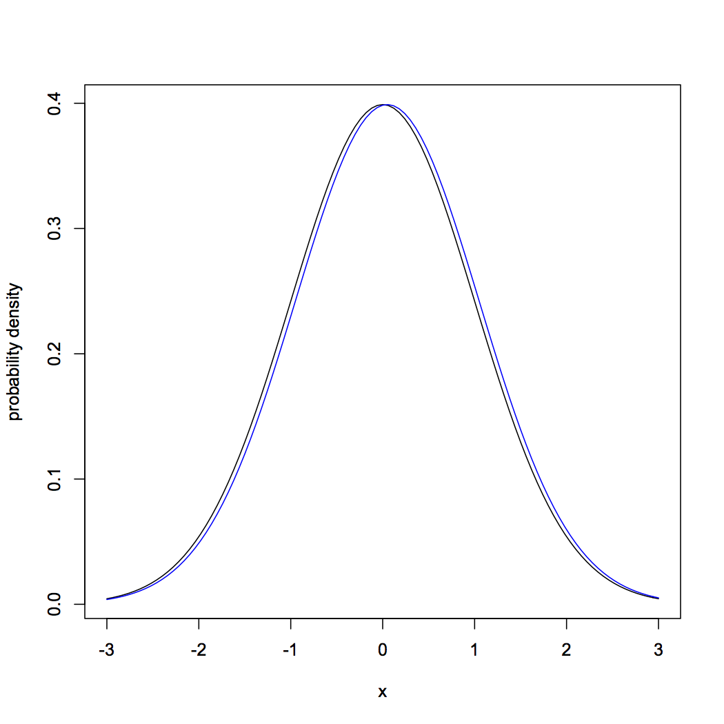
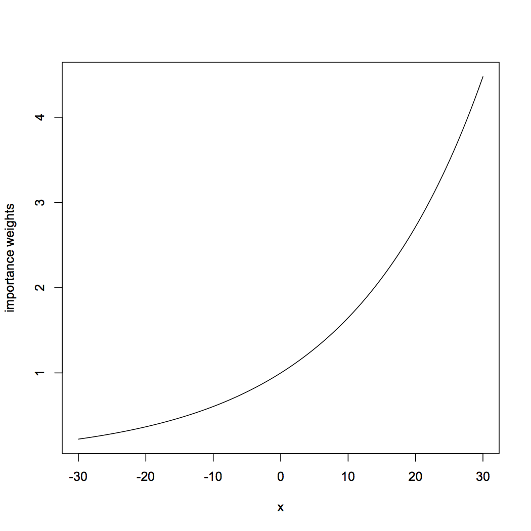
The difficulty is that the assumption of bounded weights is so incredibly restrictive as to be useless. Consider, to be concrete, two Gaussians with the same variance, and slightly shifted means:

curve(dnorm(x,0,1),from=-3,to=3,ylab="probability density") curve(dnorm(x,0.05,1),col="blue",add=TRUE)

By any reasonable standard, these are very similar distributions. However, the importance weights are unbounded:

curve(dnorm(x,0.05,1)/dnorm(x,0,1),from=-30,to=30,ylab="importance weights")

A little algebra will convince you that in this case the weight will grow without bound as \( x \rightarrow \infty \) .

One reaction would be to throw up your hands in despair, and say that nothing can be done in this situation. A little more thought, however, suggests that everything should not be hopeless here. The really huge weights, which cause the big problems, only occur for parts of the sample space which are really improbable under both distributions. It's true that the largest weight is infinite, but the average weight is quite finite, whether we compute "average" under \( Q \) or \( P \). The weights even have a finite second moment, which tells us that the central limit theorem applies. Might we not be able to use this?

At this point, the action in the Cortes et al. paper shifts to the supplemental material. As is so often the case, this is a paper in itself. As is very rarely the case, it is another good paper. (Indeed it may be more widely applicable than the main paper!)

Suppose now that we have only one distribution, but our loss-function is unbounded. It would be asking a lot to be able to control \[ \sup_{h \in H}{\left|R(h) - \hat{R}_n(h) \right|} \] when both the sample means and the true expectations could get arbitrarily large. We might, however, hope to control \[ \sup_{h \in H}{\frac{R(h) - \hat{R}_n(h)}{\sqrt{\mathbb{E}[L^2_h(X)]}}} \] since these are, to put in terms of baby stats., just Z-scores. Let's introduce the simplifying notation \[ V_h \equiv \sqrt{\mathbb{E}[L^2_h(X)]} \] for these second moments. We assume that \( V_h < \infty \) for all \( h \) , but we do not (for right now) assume that they are uniformly bounded.

The first step in controlling the fluctuations in the expected loss is to control the fluctuations in the probabilities that the loss exceeds any given threshold (Theorem 5): \[ \Pr{\left( \sup_{h\in H}{\frac{R(h) - \hat{R}_n(h)}{V_h}} > \epsilon\sqrt{2-\log{\epsilon}} \right)} \leq \Pr{\left( \sup_{h \in H, t \in \mathbb{R}}{\frac{\Pr{(L_h > t)} - \widehat{\mathrm{Pr}}(L_h > t)}{\sqrt{\Pr{(L_h > t)}}}} > \epsilon \right)} \] where \( \widehat{\mathrm{Pr}} \) is empirical probability. This is shown through combining the representation \[ \mathbb{E}{L_h(X)} = \int_{0}^{\infty}{\Pr{(L_h(X) > t)} dt} ~, \] valid for any non-negative function, with sheer trickery involving the Cauchy-Schwarz inequality. (The point of writing \( \epsilon\sqrt{2-\log{\epsilon}} \) on the left-hand side is to make the right-hand side come out simple; we'll come back to this.)

Now, notice that \( \Pr{(L_h > t)} \) is the expected value of an indicator function, \( \mathbb{E}\left[\mathbb{1}_{L_h > t}(x) \right] \), and that the corresponding empirical probability is the sample mean of the same indicator function. Cortes et al. therefore appeal to a valuable but little-known result on the relative convergence of sample proportions to probabilities, due to Anthony and Shawe-Taylor (following Vapnik), which we may phrase as follows. Let \( C \) be a set of binary classifiers, and \( G_C(n) \) be the growth function of the class, the maximum number of classifications of \( n \) points which it can realize. Further, let \( S(c) \) be the mis-classification risk of \( c \in C \), and \( \hat{S}_n(c) \) its empirical counterpart. Then \[ \Pr{\left(\sup_{c \in C}{\frac{S(c) - \hat{S}_n(c)}{\sqrt{S(c)}}} > \epsilon \right)} \leq 4 G_C(2n)e^{-n\epsilon^2 /4} \]

If, as is usual, we define the growth function of a real-valued function class as the growth function of its level sets (i.e., the sets we can get by varying \( L_h(x) > t \) over \( t \) and \( h \) ), then we combine the previous results to get \[ \Pr{\left( \sup_{h\in H}{\frac{R(h) - \hat{R}_n(h)}{V_h}} > \epsilon\sqrt{2-\log{\epsilon}} \right)} \leq 4 G_H(2n) e^{-n\epsilon^2/4} \]

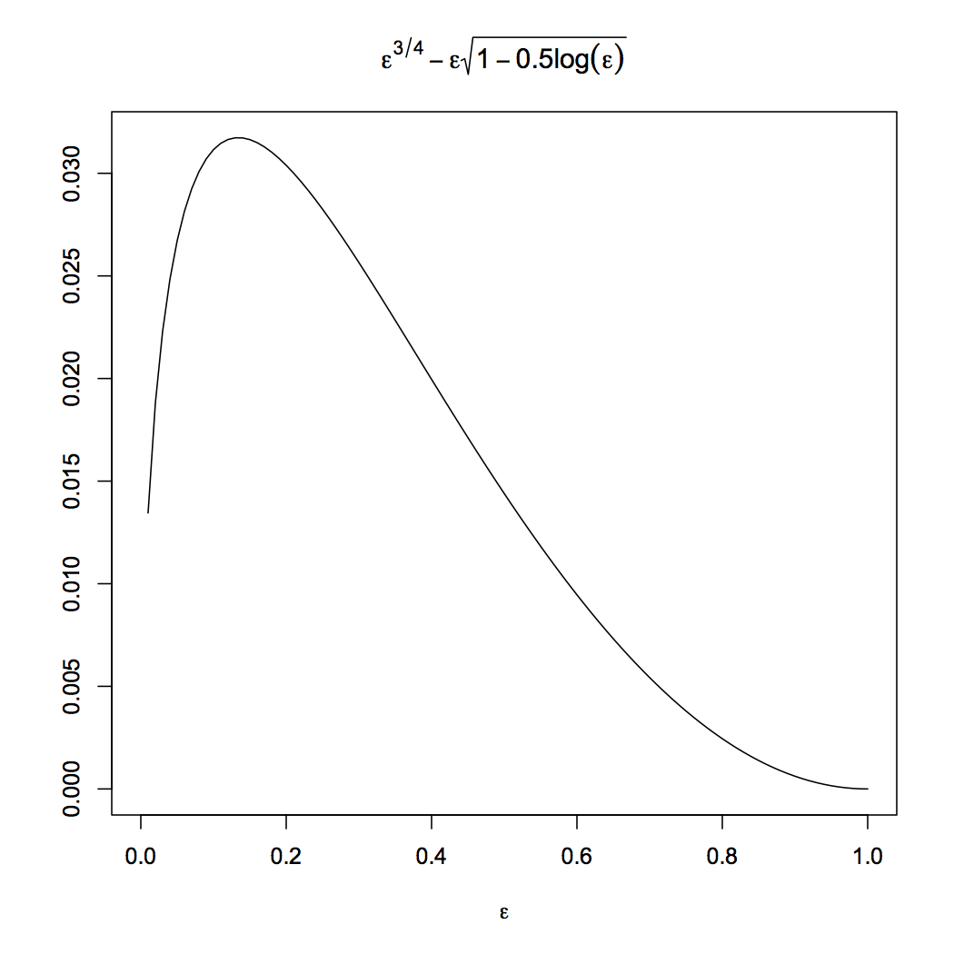
The appearance of \( \epsilon\sqrt{2-\log{\epsilon}} \) inside the probability is annoying; we would now like to shift messiness to the right-hand side of the inequality. This means setting \[ \delta = \epsilon\sqrt{2-\log{\epsilon}} \] and solving for \( \epsilon \) in terms of \( \delta \). This could actually be done in terms of the Lambert W function. Cortes et al., however, do not invoke the latter, but notice that, over the interval \( \epsilon \in [0,1] \), \[ \epsilon\sqrt{1-0.5\log{\epsilon}} \leq \epsilon^{3/4} \] but that no smaller power of \( \epsilon \) will do. (In the proof of their Corollary 1, read \( \epsilon^{\beta} \) instead of \( e^{\beta} \) throughout.) It's actually a remarkably good approximation:

curve(x^0.75 - x*sqrt(1-0.5*log(x)),from=0,to=1, xlab=expression(epsilon), ylab="", main=expression(epsilon^{3/4} - epsilon*sqrt(1-0.5*log(epsilon))))

Thus we have \[ \Pr{\left( \sup_{h\in H}{\frac{R(h) - \hat{R}_n(h)}{V_h}} > \epsilon \right)} \leq 4 G_H(2n) e^{-n\epsilon^{8/3}/4^{5/3}} \] The growth function in turn can be bounded using the Pollard pseudo-dimension, as Cortes et al. do, but the important point is that it's only polynomial in \( n \) for well-behaved function classes. This is a very nice and important result for those of us who want to use learning theory in regression, or other areas where bounded loss functions are just unnatural.

Now let us return to importance weighting. Suppose once again that our real loss function is bounded between 0 and 1, but our weights are unbounded. We have \[ \Pr{\left( \sup_{h \in H}{\frac{R(h) - \frac{1}{n}\sum_{i=1}^{n}{w(x_i) L_h(x_i)}}{\sqrt{\mathbb{E}_{Q}[w^2(X)]}}} > \epsilon \right)} \leq 4 G_{H}(2n) e^{-n\epsilon^{8/3}/4^{5/3}} \] and go from there. The quantity \( \mathbb{E}_Q[w^2(X)] \), which controls how tight the generalization error bounds are, is, as they show in some detail, related to our old friend the second-order Renyi divergence. It is this quantity which is small for our two near-by Gaussians, even though the maximum importance weights are unbounded.

Cortes et al. go on to consider variations on the importance weights, which allow some bias in the estimation of \( P \)-risk in exchange for reduced variance; this is potentially important, but more than I feel like I have energy for. I will just close by recommending footnote 1 of the supplement to connoisseurs of academic venom.

Enigmas of Chance