Three-Toed Sloth

Random-Feature Matching

\[ \newcommand{\ModelDim}{d} \]

Attention conservation notice: Academic self-promotion.

So I have a new preprint:

CRS, "A Note on Simulation-Based Inference by Matching Random Features", arxiv:2111.09220

We can, and should, do statistical inference on simulation models by adjusting the parameters in the simulation so that the values of randomly chosen functions of the simulation output match the values of those same functions calculated on the data. Results from the "state-space reconstruction" or "geometry from a time series" literature in nonlinear dynamics indicate that just \( 2\ModelDim+1 \) such functions will typically suffice to identify a model with a \( \ModelDim \)-dimensional parameter space. Results from the "random features" literature in machine learning suggest that using random functions of the data can be an efficient replacement for using optimal functions. In this preliminary, proof-of-concept note, I sketch some of the key results, and present numerical evidence about the new method's properties. A separate, forthcoming manuscript will elaborate on theoretical and numerical details.

I've been interested for a long time in methods for simulation-based inference. It's increasingly common to have generative models which are easy (or at least straightforward) to simulate, but where it's completely intractable to optimize the likelihood --- often it's intractable even to calculate it. Sometimes this is because there are lots of latent variables to be integrated over, sometimes due to nonlinearities in the dynamics. The fact that it's easy to simulate suggests that we should be able to estimate the model parameters somehow, but how?

An example: My first Ph.D. student, Linqiao Zhao, wrote her dissertation on a rather complicated model of one aspect of how financial markets work (limit-order book dynamics), and while the likelihood function existed, in some sense, the idea that it could actually be calculated was kind of absurd. What she used to fit the model instead was a very ingenious method which came out of econometrics called "indirect inference". (I learned about it by hearing Stephen Ellner present an ecological application.) I've expounded on this technique in detail elsewhere, but the basic idea is to find a second model, the "auxiliary model", which is mis-specified but easy to estimate. You then adjust the parameters in your simulation until estimates of the auxiliary from the simulation match estimates of the auxiliary from the data. Under some conditions, this actually gives us consistent estimates of the parameters in the simulation model. (Incidentally, the best version of those regularity conditions known to me are still those Linqiao found for her thesis.)

Now the drawback of indirect inference is that you need to pick the auxiliary model, and the quality of the model affects the quality of the estimates. The auxiliary needs to have at least as many parameters as the generative model, the parameters of the auxiliary need to shift with the generative parameters, and the more sensitive the auxiliary parameters are to the generative parameters, the better the estimates. There are lots of other techniques for simulation-based inference, but basically all of them turn on this same issue of needing to find some "features", some functions of the data, and tuning the generative model until those features agree between the simulations and the data. This is where people spend a lot of human time, ingenuity and frustration, as well as relying on a lot of tradition, trial-and-error, and insight into the generative model.

What occurred to me in the first week of March 2020 (i.e., just before things got really interesting) is that there might be a short-cut which avoided the need for human insight and understanding. That week I was teaching kernel methods and random features in data mining, and starting to think about how I wanted to revise the material on simulation-based inference for my "data over space and time" in the fall. The two ideas collided in my head, and I realized that there was a lot of potential for estimating parameters in simulation models by matching random features, i.e., random functions of the data. After all, if we think of an estimator as a function from the data to the parameter space, results in Rahimi and Recht (2008) imply that a linear combination of \( k \) random features will, with high probability, give an \( O(1/\sqrt{k}) \) approximation to the optimal function.

Having had that brainstorm, I then realized that there was a good reason to think a fairly small number of random features would be enough. As we vary the parameters in the generative model, we get different distributions over the observables. Actually working out that distribution is intractable, that's why we're doing simulation-based inference in the first place, but it'll usually be the case that the distribution changes smoothly with the generative parameters. That means that if there are \( \ModelDim \) parameters, the space of possible distributions is also just \( \ModelDim \)-dimensional --- the distributions form a \( \ModelDim \)-dimensional manifold.

And, as someone who was raised in the nonlinear dynamics sub-tribe of physicists, \( \ModelDim \)-dimensional manifolds remind me about state-space reconstruction and geometry from a time series and embedology. Specifically, back behind the Takens embedding theorem used for state-space reconstruction, there lies the Whitney embedding theorem. Suppose we have a \( \ModelDim \)-dimensional manifold \( \mathcal{M} \), and we consider a mapping \( \phi: \mathcal{M} \mapsto \mathbb{R}^k \). Suppose that each coordinate of \( \phi \) is \( C^1 \), i.e., continuously differentiable. Then once \( k=2\ModelDim \), there exists at least one \( \phi \) which is a diffeomorphism, a differentiable, 1-1 mapping of \( \mathcal{M} \) to \( \mathbb{R}^k \) with a differentiable inverse (on the image of \( \mathcal{M} \)). Once \( k \geq 2\ModelDim+1 \), diffeomorphisms are "generic" or "typical", meaning that they're the most common sort of mapping, in a certain topological sense, and dense in the set of all mappings. They're hard to avoid.

In time-series analysis, we use this to convince ourselves that taking \( 2\ModelDim+1 \) lags of some generic observable of a dynamical system will give us a "time-delay embedding", a manifold of vectors which is equivalent, up to a smooth change of coordinates, to the original, underlying state-space. What I realized here is that we should be able to do something else: if we've got \( \ModelDim \) parameters, and distributions change smoothly with parameters, then the map between the parameters and the expectations of \( 2\ModelDim+1 \) functions of observables should, typically or generically, be smooth, invertible, and have a smooth inverse. That is, the parameters should be identifiable from those expectations, and small errors in the expectations should track back to small errors in the parameters.

Put all this together: if you've got a \( \ModelDim \)-dimensional generative model, and I can pick \( 2\ModelDim+1 \) random functions of the observables which converge on their expectation values, I can get consistent estimates of the parameters by adjusting the \( \ModelDim \)-generative parameters until simulation averages of those features match the empirical values.

Such was the idea I had in March 2020. Since things got very busy after that (as you might recall), I didn't do much about this except for reading and re-reading papers until the fall, when I wrote it up as grant proposal. I won't say where I sent it, but I will say that I've had plenty of proposals rejected (those are the breaks), but never before have I had feedback from reviewers which made me go "Fools! I'll show them all!". Suitably motivated, I have been working on it furiously all summer and fall, i.e., wrestling with my own limits as a programmer.

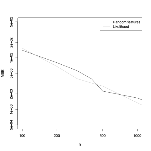
But now I can say that it works. Take the simplest thing I could possibly want to do, estimating the location \( \theta \) of a univariate, IID Gaussian, \( \mathcal{N}(\theta,1) \). I make up three random Fourier features, i.e., I calculate \[ F_i = \frac{1}{n}\sum_{t=1}^{n}{\cos{(\Omega_i X_t + \alpha_i)}} \] where I draw \( \Omega_i \sim \mathcal{N}(0,1) \) independently of the data, and \( \alpha_i \sim \mathrm{Unif}(-\pi, \pi) \). I calculate \( F_1, F_2, F_3 \) on the data, and then use simulations to approximate their expectations as a function of \( \theta \) for different \( \theta \). I return as my estimate of \( \theta \) whatever value minimizes the squared distance from the data in these three features. And this is what I get for the MSE:

OK, it doesn't fail on the simplest possible problem --- in fact it's actually pretty close to the performance of the MLE. Let's try something a bit less well-behaved, say having \( X_t \sim \theta + T_5 \), where \( T_5 \) is a \( t \)-distributed random variable with 5 degrees of freedom. Again, it's a one-parameter location family, and the same 3 features I used for the Gaussian family work very nicely again:

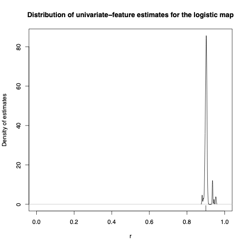
OK, it can do location families. Since I was raised in nonlinear dynamics, let's try a deterministic dynamical system, specifically the logistic map: \[ S_{t+1} = 4 r S_t(1-S_t) \] Here the state variable \( S_t \in [0,1] \), and the parameter \( r \in [0,1] \) as well. Depending on the value of \( r \), we get different invariant distributions over the state-space. If I sampled \( S_1 \) from that invariant distribution, this'd be a stationary and ergodic stochastic process; if I just make it \( S_1 \sim \mathrm{Unif}(0,1) \), it's still ergodic but only asymptotically stationary. If I used the same 3 random Fourier features, well, this is the distribution of estimates from time series of length 100, when the true \( r=0.9 \), so the dynamics are chaotic:

I get very similar results if I use random Fourier features that involve two time points, i.e., time-averages of \( \cos{(\Omega_{i1} X_{t} + \Omega_{i2} X_{t-1} + \alpha+i)} \), but I'll let you look at those in the paper, and also at how the estimates improve when I increase the sample size.

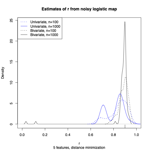
Now I try estimating the logistic map, only instead of observing \( S_t \) I observed \( Y_t = S_t + \mathcal{N}(0, \sigma^2) \). The likelihood function is no longer totally pathological, but it's also completely intractable to calculate or optimize. But matching 5 (\( =2\times 2 + 1 \)) random Fourier features works just fine:

 

At this point I think I have enough results to have something worth sharing, though there are of course about a bazillion follow-up questions to deal with. (Other nonlinear features besides cosines! Non-stationarity! Spatio-temporal processes! Networks! Goodness-of-fit testing!) I will be honest that I partly make this public now because I'm anxious about being scooped. (I have had literal nightmares about this.) But I also think this is one of the better ideas I've had in years, and I've been bursting to share.

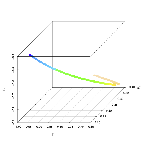
As \( r \) in the logistic map varies from 0 (dark blue) to 1 (light pink), time-averages of 3 random Fourier features trace out a smooth, one-dimensional manifold in three-dimensional space. Different choices of random features would give different embeddings of the parameter space, butthat three random features give an embedding is generic.

Update, 21 June 2022: a talk on this, in two days time.

Update, 12 September 2023: a funded grant.

Self-centered; Enigmas of Chance