After long, long journeys, in one case going back to 2003, some papers have come out. Alphabetically by distinguished co-authors:
I could be rightbut many of them at least pretend to care about the truth of their claims, so I piously hope that in the fullness of time the community of inquirers will come around to using reliable methods. In which regard I am gratified, but also astonished, to see that this is already the most-cited paper I've contributed to, by such a large margin that it's unlikely anything else I do will ever rival it.
I could be wrong
I feel nice when I sing this song
Other output: my first hemi-demi-semi-co-supervised student graduating with his doctorate (a fine piece of work I wish I could link to); a paper draft finished and sitting on a collaborator's desk (no pressure!); the homophily paper is almost finished (I need to speed up some simulations and cut out most of the jokes); half-a-dozen referee reports of my own (a deliberate new low; made easier by boycotting Elsevier); five papers edited for Annals of Applied Statistics (a new high); nine lectures newly written or massively revised for 36-350; all the problem sets for 350 re-worked and much better; three books reviewed for American Scientist (and a whole bunch of mini-reviews for nowhere in particular).
On the other hand, no chapters finished for Statistical Analysis of Complex Systems; three very patient collaborators in different parts of Manhattan waiting for me to turn things around; and one project which has been accreting since 2007 really needs to be cut and polished into some papers. Resolution for next year: more papers.
Self-Centered; Enigmas of Chance; Complexity; Power Laws; Minds, Brains, and Neurons
Posted by crshalizi at December 31, 2009 18:45 | permanent link
Attention conservation notice: 2100 words on parallels between statistical hypothesis testing and Jamesian pragmatism; an idea I've been toying with for a decade without producing anything decisive or practical. Contains algebraic symbols and long quotations from ancient academic papers. Also some history-of-ideas speculation by someone who is not a historian.
When last we saw the Neyman-Pearson lemma, we were looking at how to tell whether a data set x was signal or noise, assuming that we know the statistical distributions of noise (call it p) and the distribution of signals (q). There are two kinds of mistake we can make here: a false alarm, saying "signal" when x is really noise, and a miss, saying "noise" when x is really signal. What Neyman and Pearson showed is that if we fix on a false alarm rate we can live with (a probability of mistaking noise for signal; the "significance level"), there is a unique optimal test which minimizes the probability of misses --- which maximizes the power to detect signal when it is present. This is the likelihood ratio test, where we say "signal" if and only if q(x)/p(x) exceeds a certain threshold picked to control the false alarm rate.
The Neyman-Pearson lemma comes from their 1933 paper; but the distinction between the two kinds of errors, which is clearly more fundamental. Where does it come from?
The first place Neyman and/or Pearson use it, that I can see, is their 1928 paper (in two parts), where it's introduced early and without any fanfare. I'll quote it, but with some violence to their notation, and omitting footnoted asides (from p. 177 of part I; "Hypothesis A" is what I'm calling "noise"):
Setting aside the possibility that the sampling has not been random or that the population has changed during its course, x must either have been drawn randomly from p or from q, where the latter is some other population which may have any one of an infinite variety of forms differing only slightly or very greatly from p. The nature of the problem is such that it is impossible to find criteria which will distinguish exactly between these alternatives, and whatever method we adopt two sources of error must arise:The 1928 paper goes on to say that, intuitively, it stands to reason that the likelihood ratio is the right way to accomplish this. The point of the 1933 paper is to more rigorously justify the use of the likelihood ratio (hence the famous "lemma", which is really not set off as a separate lemma...). Before unleashing the calculus of variations, however, they warm up with some more justification (pp. 295--296 of their 1933):
- Sometimes, when Hypothesis A is rejected, x will in fact have been drawn from p.
- More often, in accepting Hypothesis A, x will really have been drawn from q.
In the long run of statistical experience the frequency of the first source of error (or in a single instance its probability) can be controlled by choosing as a discriminating contour, one outside which the frequency of occurrence of samples from p is very small — say, 5 in 100 or 5 in 1000. In the density space such a contour will include almost the whole weight of the field. Clearly there will be an infinite variety of systems from which it is possible to choose a contour satisfying such a condition....
The second source of error is more difficult to control, but if wrong judgments cannot be avoided, their seriousness will at any rate be diminished if on the whole Hypothesis A is wrongly accepted only in cases where the true sampled population, q, differs but slightly from p.
Let us now for a moment consider the form in which judgments are made in practical experience. We may accept or we may reject a hypothesis with varying degrees of confidence; or we may decide to remain in doubt. But whatever conclusion is reached the following position must be recognized. If we reject H0, we may reject it when it is true; if we accept H0, we may be accepting it when it is false, that is to say, when really some alternative Ht is true. These two sources of error can rarely be eliminated completely; in some cases it will be more important to avoid the first, in others the second. We are reminded of the old problem considered by LAPLACE of the number of votes in a court of judges that should be needed to convict a prisoner. Is it more serious to convict an innocent man or to acquit a guilty? That will depend upon the consequences of the error; is the punishment death or fine; what is the danger to the community of released criminals; what are the current ethical views on punishment? From the point of view of mathematical theory all that we can do is to show how the risk of the errors may be controlled and minimised. The use of these statistical tools in any given case, in determining just how the balance should be struck, must be left to the investigator.(Neither Laplace nor LAPLACE, are mentioned in their 1928 paper.)
Let's step back a little bit to consider the broader picture here. We have a question about what the world is like --- which of several conceivable hypotheses is true. Some hypotheses are ruled out on a priori grounds, others because they are incompatible with evidence, but that still leaves more than one admissible hypothesis, and the evidence we have does not conclusively favor any of them. Nonetheless, we must chose one hypothesis for purposes of action; at the very least we will act as though one of them is true. But we may err just as much through rejecting a truth as through accepting a falsehood. The two errors are symmetric, but they are not the same error. In this situation, we are advised to pick a hypothesis based, in part, on which error has graver consequences.
This is precisely the set-up of William James's "The Will to Believe". (It's easily accessible online, as are summaries and interpretations; for instance, an application to current controversies by Jessa Crispin.) In particular, James lays great stress on the fact that what statisticians now call Type I and Type II errors are both errors:
There are two ways of looking at our duty in the matter of opinion, — ways entirely different, and yet ways about whose difference the theory of knowledge seems hitherto to have shown very little concern. We must know the truth; and we must avoid error, — these are our first and great commandments as would-be knowers; but they are not two ways of stating an identical commandment, they are two separable laws. Although it may indeed happen that when we believe the truth A, we escape as an incidental consequence from believing the falsehood B, it hardly ever happens that by merely disbelieving B we necessarily believe A. We may in escaping B fall into believing other falsehoods, C or D, just as bad as B; or we may escape B by not believing anything at all, not even A.Believe truth! Shun error! — these, we see, are two materially different laws; and by choosing between them we may end by coloring differently our whole intellectual life. We may regard the chase for truth as paramount, and the avoidance of error as secondary; or we may, on the other hand, treat the avoidance of error as more imperative, and let truth take its chance. Clifford ... exhorts us to the latter course. Believe nothing, he tells us, keep your mind in suspense forever, rather than by closing it on insufficient evidence incur the awful risk of believing lies. You, on the other hand, may think that the risk of being in error is a very small matter when compared with the blessings of real knowledge, and be ready to be duped many times in your investigation rather than postpone indefinitely the chance of guessing true. I myself find it impossible to go with Clifford. We must remember that these feelings of our duty about either truth or error are in any case only expressions of our passional life. Biologically considered, our minds are as ready to grind out falsehood as veracity, and he who says, "Better go without belief forever than believe a lie!" merely shows his own preponderant private horror of becoming a dupe. He may be critical of many of his desires and fears, but this fear he slavishly obeys. He cannot imagine any one questioning its binding force. For my own part, I have also a horror of being duped; but I can believe tbat worse things tban being doped may happen to a man in this world: so Clifford's exhortation has to my ears a thoroughly fantastic sound. It is like a general informing his soldiers that it is better to keep out of battle forever than to risk a single wound. Not so are victories either over enemies or over nature gained. Our errors are surely not such awfully solemn things. In a world where we are so certain to incur them in spite of all our caution, a certain lightness of heart seems healthier than this excessive nervousness on their behalf. At any rate, it seems the fittest thing for the empiricist philosopher.
From here the path to James's will to believe is pretty clear, at least in the form he advocated it, which is that of picking among hypotheses which are all "live"*, and where some choice must be made among them. What I am interested in, however, is not the use James made of this distinction, but simply the fact that he made it.
So far as I have been able to learn, no one drew this distinction between seeking truth and avoiding error before James, or if they did, they didn't make anything of it. (Even for Pascal in his wager, the idea that believing in Catholicism if it is false might be bad doesn't register.) Yet this is just what Neyman and Pearson were getting at, thirty-odd years later. There is no mention of James in these papers, or indeed of any other source. They present the distinction as though it were obvious, though eight decades of subsequent teaching experience shows its anything but. Neyman and Pearson were very interested in the foundations of statistics, but seem to have paid no attention to earlier philosophers, except for the arguable case of Pearson's father Karl and his Grammar of Science (which does not seem to mention James). Yet there it is. It really looks like two independent inventions of the whole scheme for judging hypotheses.
My prejudices being what they are, I am much less inclined to think that James illuminates Neyman and Pearson than the other way around. James was, so to speak, arguing that we should trade significance — the risk of mistaking noise for signal — for power, finding some meaningful signal in the "blind molecular chaos" of the physical universe. Granting that there is a trade-off here, however, one has to wonder about how stark it really is (cf.), and whether his will-to-believe is really the best way to handle it. Neyman and Pearson suggest we should look for a procedure for resolving metaphysical questions which maximizes the ability to detect larger meanings for a given risk of seeing faces in clouds — and would let James and Clifford set their tolerance for that risk to their own satisfaction. Of course, any such procedure would have to squarely confront the fact that there may be no way of maximizing power against multiple alternatives simultaneously...
The extension to confidence sets, consisting of all hypotheses not rejected by suitably powerful tests (per Neyman 1937) is left as an exercise to the reader.
*: As an example of a "dead" hypothesis, James gives believing in "the Mahdi", presumably Muhammad Ahmad ibn as-Sayyid Abd Allah. I'm not a Muslim, and those of my ancestors who were certainly weren't Mahdists, but this was still a "What do you mean 'we', white man?" moment in my first reading of the essay. To be fair, James gives me many fewer such moments than most of his contemporaries.
Manual trackback: Brad DeLong.
Posted by crshalizi at December 28, 2009 00:08 | permanent link
Attention conservation notice: 1000 words on a short probability problem. Several hobby-horses get to take turns around the yard.
Wolfgang at Mostly Harmless poses a problem (I've lightly tweaked the notation):
Consider a random process X(t) which generates a series of 0s and 1s, but many more 0s because the probability for X(t) = 1 decreases with t as 2-t.Now assume that we encounter this process not knowing 'how far we are already', in other words we don't know the value of t. The question is: "What is the probability to get a 1?"
Unfortunately there are two ways to answer this question. The first calculates the 'expectation value', as a physicist would call it, or 'the mean' as a statistician would put it, which is zero.
In other words, we sum over all possible t with equal weight and have to consider s = sum( 2-t ) with t = 1, 2, ... N; It is not difficult to see that s = 1/2 + 1/4 + ... equals 1.
The answer is therefore Pr(X=1) = s/N = 1/N and because N is infinite (the process never ends) we get Pr(X=1) = 0.
The second answer simply looks at the definition of the process and points out that Pr(X=1) = 2-T, where T is the current value of t. Although we don't know T it must have some finite value and it is obvious that Pr(X=1) > 0.
So which one is it, Pr(X=1) = 0 or Pr(X=1) > 0?
Fatwa: The second answer is correct, and the first is wrong.
Discussion: This is a cute example of the weirdness which results when we attempt to put uniform distributions on infinite spaces, even in the simplest possible case of the positive integers. The first way of proceeding assumes that the notion of a uniform probability distribution on the natural numbers makes sense, and that it obeys the same rules as an ordinary probability distribution. Unfortunately, these two requirements are incompatible. This is because ordinary probability distributions are countably additive. We are all familiar with the fact that probability adds across disjoint events: Pr(X= 0 or 1) = Pr(X=0)+Pr(X=1). Moreover, we are all comfortable with the idea that this holds for more than two events. The probability that X first =1 by time 3 is the sum of the probability of the first 1 being at time t=1, plus it being at t=2, plus it being at t=3. Carrying this out to any finite collection of disjoint events is called finite additivity. However, as I said, probability measures are ordinarily required to be countably additive, meaning that this holds even for a countable infinity of disjoint events.
And here we have trouble. The natural numbers are (by definition!) countable, so the probability of all integers is the sum of the probability of each integer,
Now, there are such things as finitely-additive probability measures, but they are rather weird beasts. To specify one of them on the integers, for example, it's not enough to give the probability of each integer (as it is for a countably-additive measure); that only pins down the probability of finite sets, and sets whose complements are finite. It does not, for example, specify the probability of the even numbers. There turn out to be several different ways of defining uniform distributions on the natural numbers, which are not equivalent. Under all of them, however, any finite set must have probability zero, and so at a random time T, it is almost certain that Pr(X(T)=1) is less than any real number you care to name. Hence, the expectation value of this random probability is indeed zero.
(Notice, however, that if I try to calculate the expectation value of any function f(t) by taking a probability-weighted sum over values of t, as the first answer does, I will get the answer 0 when T follows a uniform finitely-additive measure, even if f(t)=1 for all t. The weighted-sum-of-arguments definition of expectation — the one reminiscent of Riemann integrals — does not work for these measures. Instead one must use a Lebesgue-style definition, where one takes a weighted sum of the values of the function, the weights being the measures of the sets giving those values. [More exactly, one partitions the range of f and takes the limit as the partition becomes finer and finer.] The equivalence of the summing over the domain and summing over the range turns on, precisely, countable additivity. The argument in the previous paragraph shows that here this expectation value must be less than any positive number, yet not negative, hence zero.)
Finitely-additive probability measures are profoundly weird beasts, though some of my colleagues have what I can only consider a perverse affection for them. On the other hand, attempts to construct a natural countably-additive analog of a uniform distribution on infinite sets have been universally unsuccessful; this very much includes the maximum entropy approach. The project of giving ignorance a unique representation as a probability measure is, IMSAO, a failure. If one picks some countably-additive prior distribution over the integers, however, then at least one value of t must have strictly positive probability, and the expectation value of Pr(X(T)=1) is positive, though how big it is will depend on the prior distribution. (As usual, the role of a Bayesian prior distribution is to introduce bias so as to reduce variance.) Alternately, one simply follows the second line of reasoning and concludes that, no matter what t might be, the probability is positive.
Posted by crshalizi at December 08, 2009 10:55 | permanent link
My lesson-plan having survived first contact with
the enemy students, it's time to start posting the lecture
handouts & c. This page will be updated as the semester goes on; the RSS
feed for it should be here.
The class homepage has more
information.
Homework 1, due 4 September: assignment, R, data; solutions
Homework 2, due 11 September: assignment; solutions text and R code
Homework 3, due 18 September: assignment; solutions
Homework 4, due 25 September: assignment; solutions
Pre-midterm review (12 October): highlights of the course to date; no
handout.
MIDTERM (14
October): exam, solutions
Homework 5, due 23 October: assignment; solutions
Homework 6, due Friday, 30 October: assignment, data set; solutions
Homework 7, due Friday, 6 November: assignment; solutions: text and code
Homework 8, due 5 pm on Monday, 16 November: assignment; solutions; R for solutions
Homework 9, due at 5 pm on Monday, 30 November: assignment
Take-home final exam, due 15 December: assignment; data sets: expressdb_cleaned (20 Mb), HuIyer_TFKO_expression (20 Mb). With great thanks to Dr. Timothy Danford.
Posted by crshalizi at December 05, 2009 14:39 | permanent link
Posted by crshalizi at November 30, 2009 23:59 | permanent link
Attention conservation notice: Unskillful nattering about pop-culture ephemera.For the sake of my own sanity, I prefer to remain ignorant of the occult processes by which the direct mail gods decide to which catalogues to send to which people. (There's too much dynamic programming involved.) Today, for instance, they decided to inflict upon me the official Barbie doll spring 2010 collection preview, and like a fool I couldn't resist looking through it. Thus my life is made that much worse by learning that there is a Joan Jett Barbie doll. (I thought about embedding an image, but in this case pain shared is not pain eased.) I think I finally grasp what people mean when they talk about later cultural products assaulting parts of their childhood, in this case one I didn't even realize I valued.
Manual trackback: Mostly Harmless
Posted by crshalizi at November 24, 2009 19:27 | permanent link
A number of people have asked for my slides from the MERSIH conference the other week. So, here they are. (Anyone who was at my talk at SFI about a year ago will recognize the title, and much of the content.) I'm presently turning this into a proper manuscript, so comments are welcome. Please don't rip it off; I'll become very cross and may even hold my breath until I turn blue and pass out, and won't you be sorry then?
Manual trackback: Cognition and Culture
Posted by crshalizi at November 21, 2009 18:32 | permanent link
In which the starry heavens above submit to statistical analysis:
Enigmas of Chance; The Eternal Silence of These Infinite Spaces; Physics
Posted by crshalizi at November 19, 2009 12:02 | permanent link
Attention conservation notice: Of no use to you unless (1) you want to know what statisticians do at search-engine companies and (2) you are in Pittsburgh.
As always, the talk is free and open to the public.
Posted by crshalizi at November 13, 2009 15:09 | permanent link
Attention conservation notice: Quasi-teaching note giving an economic interpretation of the Neyman-Pearson lemma on statistical hypothesis testing.
Suppose we want to pick out some sort of signal from a background of noise. As every schoolchild knows, any procedure for doing this, or test, divides the data space into two parts, the one where it says "noise" and the one where it says "signal".* Tests will make two kinds of mistakes: they can can take noise to be signal, a false alarm, or can ignore a genuine signal as noise, a miss. Both the signal and the noise are stochastic, or we can treat them as such anyway. (Any determinism distinguishable from chance is just insufficiently complicated.) We want tests where the probabilities of both types of errors are small. The probability of a false alarm is called the size of the test; it is the measure of the "say 'signal'" region under the noise distribution. The probability of a miss, as opposed to a false alarm, has no short name in the jargon, but one minus the probability of a miss — the probability of detecting a signal when it's present — is called power.
Suppose we know the probability density of the noise p and that of the signal is q. The Neyman-Pearson lemma, as many though not all schoolchildren know, says that then, among all tests off a given size s, the one with the smallest miss probability, or highest power, has the form "say 'signal' if q(x)/p(x) > t(s), otherwise say 'noise'," and that the threshold t varies inversely with s. The quantity q(x)/p(x) is the likelihood ratio; the Neyman-Pearson lemma says that to maximize power, we should say "signal" if its sufficiently more likely than noise.
The likelihood ratio indicates how different the two distributions — the two hypotheses — are at x, the data-point we observed. It makes sense that the outcome of the hypothesis test should depend on this sort of discrepancy between the hypotheses. But why the ratio, rather than, say, the difference q(x) - p(x), or a signed squared difference, etc.? Can we make this intuitive?
Start with the fact that we have an optimization problem under a constraint. Call the region where we proclaim "signal" R. We want to maximize its probability when we are seeing a signal, Q(R), while constraining the false-alarm probability, P(R) = s. Lagrange tells us that the way to do this is to minimize Q(R) - t[P(R) - s] over R and t jointly. So far the usual story; the next turn is usually "as you remember from the calculus of variations..."
Rather than actually doing math, let's think like economists. Picking the set R gives us a certain benefit, in the form of the power Q(R), and a cost, tP(R). (The ts term is the same for all R.) Economists, of course, tell us to equate marginal costs and benefits. What is the marginal benefit of expanding R to include a small neighborhood around the point x? Just, by the definition of "probability density", q(x). The marginal cost is likewise tp(x). We should include x in R if q(x) > tp(x), or q(x)/p(x) > t. The boundary of R is where marginal benefit equals marginal cost, and that is why we need the likelihood ratio and not the likelihood difference, or anything else. (Except for a monotone transformation of the ratio, e.g. the log ratio.) The likelihood ratio threshold t is, in fact, the shadow price of statistical power.
I am pretty sure I have not seen or heard the Neyman-Pearson lemma explained marginally before, but in retrospect it seems too simple to be new, so pointers would be appreciated.
Manual trackback: John Barrdear
Updates: Thanks to David Kane for spotting a typo.
*: Yes, you could have a randomized test procedure, but the situations where those actually help pretty much define "boring, merely-technical complications."
Posted by crshalizi at November 08, 2009 03:06 | permanent link
My old Blosxom installation (v. 2.0.2), after several years of working nicely, is growing increasingly cranky, and mulishly refusing to generate or update posts as the whim takes it. (I am not sure how much kicking and shoving it will need to produce this.) I'd appreciate a pointer to something which works similarly, but does work: I write posts in plain HTML in Emacs and drop them in a directory; it makes them look nice. If it handles tags and/or LaTeX nicely, so much the better.
Posted by crshalizi at November 04, 2009 19:34 | permanent link
Books to Read While the Algae Grow in Your Fur; Enigmas of Chance; Scientifiction and Fantastica; Pleasures of Detection, Portraits of Crime; Writing for Antiquity; The Great Transformation; Physics; Complexity; Cthulhiana
Posted by crshalizi at October 31, 2009 23:59 | permanent link
Attention conservation notice: Idle economic musings of a non-economist. Sparked by recent developments, but if you're interested in that you'd be better off elsewhere.
The usual libertarian story about professional licensing requirements — e.g., requiring someone who wants to practice medicine to go to medical school and pass exams, on pain of fines or jail — is that these are simply professionals conspiring in restraint of trade. Licensing simply erects a barrier to entry into the market for medical services, restricting supply and driving up price. Eliminate it, they say, and supply will expand and prices fall.
This presumes, however, that the demand for unlicensed professionals will be equal to the demand for licensed ones. It seems to me very easy to tell a "market for lemons" story here: someone in the market for professional services generally knows very little about how skilled various potential providers actually are. The sellers, however, generally know a lot about their own skill level, or at least more than the potential clients do. (There are no doubt exceptions, such as sincere quacks and the Dunning-Kreuger effect, but I don't think matters for the story.) This is the classic asymmetric information problem from Akerlof, with the usual result: the skilled providers demand more, but the clients have no way of telling them from the unskilled ones, so the only equilibrium is for only unskilled providers to be on the market and for trade to be depressed, or indeed absent. By putting a floor on the incompetence of professionals, licensing requirements stop the unraveling of the market and increase demand. They get us out of the market for lemons.
This occurred to me the other day, but it's obvious enough that I'm sure someone wrote it up long ago; where? (And did I read it and forget about it?)
(After-notes: 1. Of course, having told the story I have no idea if it's true of actual markets for professional services; learning that would require rather delicate empirical investigations. Checking the restraint-of-trade fable from Milton Friedman would, naturally, require those same investigations. 2. This doesn't rationalize why professions should be so largely self-governing, nor does it rule out the idea that some licensing requirements are counter-productive barriers to entry. 3. Replacing professional certification with some sort of market-based entity telling consumers about the quality of professional service-sellers won't work, for all the usual reasons that competitive markets are incapable of adequately providing information — to say nothing of the difficulty of telling whether the raters know what they're talking about. 4. Universities are accredited because students and parents would otherwise be in a market for lemons. Universities themselves, however, can tell how skilled those selling academic services are — or at least they're supposed to have that ability. 5. I should re-read Phil Agre on the professionalization of everything and see if it holds up.)
Posted by crshalizi at October 13, 2009 22:26 | permanent link
My review of Justin Fox's Myth of the Rational Market in American Scientist is out. (Shorter me: read the book.) Sometime soon I'll put up a version with links, which alas don't work in print.
Manual trackback: 3 Quarks Daily
Posted by crshalizi at October 09, 2009 00:54 | permanent link
"They [= the Steelers] are like this utterly adorable, totally hot girl next door, who you suddenly realize is everything you've ever wanted in a football team — I mean, girlfriend."
Posted by crshalizi at October 08, 2009 23:00 | permanent link
Attention conservation notice: Only of interest if you (1) care about specifying probability distributions on infinite-dimensional spaces for use in nonparametric Bayesian inference, and (2) are in Pittsburgh.
The CMU statistics department sponsors an annual distinguished lecture series in memory of our sainted founder, Morris H. DeGroot. This year, the lecturer is Michael Jordan. (I realize that's a common name; I mean the one my peers and I wanted to be when we grew up.)
Update: I counted over 210 people in the audience.
Posted by crshalizi at October 08, 2009 15:02 | permanent link
Attention conservation notice: Only of interest if you (1) care about statistical learning in high-dimensional spaces and (2) are in Pittsburgh.
Since manifold learning has been on my mind this week, owing to trying to teach it in data-mining, I am extra pleased by the scheduling of this talk:
As always, the seminar is free and open to the public.
Posted by crshalizi at October 08, 2009 15:01 | permanent link
Having vowed two weeks ago to post something positive at least once a week, I missed last week, with the excuse of being back in Ann Arbor for the celebration of John Holland's 80th birthday at the Center for the Study of Complex Systems. There was no time to post, or even to see everyone I wanted to, but I did actually start writing something about Holland's scientific work, only to realize yesterday I was merely engaged in self-plagiarism, from this, this and this, and probably other things I'd written too, because reading Holland has quite profoundly shaped my thinking. So I'll just point you to the back-catalogue, as it were, and get back to revising a paper I'd never have written if I hadn't read Adaptation in Natural and Artificial Systems.
(So long as I'm talking about the workshop, and without any slight to the other presentations, the neatest work was that by Stephanie Forrest et al. on using genetic programming to evolve bug fixes.)
Posted by crshalizi at October 05, 2009 14:30 | permanent link
See you in Whistler?
Analyzing Networks and Learning with Graphs
a workshop in conjunction with23nd Annual Conference on Neural Information Processing Systems (NIPS 2009)
December 11 or 12, 2009 (exact date TBD) Whistler, BC, CanadaDeadline for Submissions: Friday, October 30, 2009
Notification of Decision: Monday, November 9, 2009Overview:
Recent research in machine learning and statistics has seen the proliferation of computational methods for analyzing networks and learning with graphs. These methods support progress in many application areas, including the social sciences, biology, medicine, neuroscience, physics, finance, and economics.
The primary goal of the workshop is to actively promote a concerted effort to address statistical, methodological and computational issues that arise when modeling and analyzing large collection of data that are largely represented as static and/or dynamic graphs. To this end, we aim at bringing together researchers from applied disciplines such as sociology, economics, medicine and biology, together with researchers from more theoretical disciplines such as mathematics and physics, within our community of statisticians and computer scientists. Different communities use diverse ideas and mathematical tools; our goal is to to foster cross-disciplinary collaborations and intellectual exchange.
Presentations will include novel graph models, the application of established models to new domains, theoretical and computational issues, limitations of current graph methods and directions for future research.
Online Submissions
We welcome the following types of papers:All submissions will be peer-reviewed; exceptional work will be considered for oral presentation. We encourage authors to emphasize the role of learning and its relevance to the application domains at hand. In addition, we hope to identify current successes in the area, and will therefore consider papers that apply previously proposed models to novel domains and data sets.
- Research papers that introduce new models or apply established models to novel domains,
- Research papers that explore theoretical and computational issues, or
- Position papers that discuss shortcomings and desiderata of current approaches, or propose new directions for future research.
Submissions should be 4-to-8 pages long, and adhere to NIPS format. Please email your submissions to: nipsgraphs2009 [at] gmail [dot] com
Workshop Format
This is a one-day workshop. The program will feature invited talks, poster sessions, poster spotlights, and a panel discussion. All submissions will be peer-reviewed; exceptional work will be considered for oral presentation. More details about the program will be announced soon.Organizers
- Edoardo Airoldi, Harvard University
- Jon Kleinberg, Cornell University
- Jure Leskovec, Stanford University
- Josh Tenenbaum, MIT
Posted by crshalizi at October 02, 2009 10:24 | permanent link
Books to Read While the Algae Grow in Your Fur; Enigmas of Chance; The Dismal Science; Pleasures of Detection, Portraits of Crime; Scientifiction and Fantastica; Philosophy; Writing for Antiquity; The Great Transformation
Posted by crshalizi at September 30, 2009 23:59 | permanent link
It would be wrong to say that Judea Pearl knows more about causal inference than anyone else — I can think of some rivals very close to where I'm writing this — but he certainly knows a lot, and has worked tirelessly to formulate and spread the modern way of thinking about the subject, centered around graphical models and their associated structural equations. I remember spending many happy hours with his book Causality when it came out in 2000, and look forward to spending more with the new edition, which is making its way to me through the mail now. In the meanwhile, however, there is what he describes as "A new survey paper, gently summarizing everything I know about causation (in only 43 pages)":
The paper assumes a reader who's reasonably well-grounded in statistics, though not necessarily in the causal-inference literature. (Of such readers, I imagine applied economists might have more unlearning to do than most, because they will keep asking "but when do I start estimating beta?") It's not ideally calibrated for an reader coming from, say, machine learning.
One theme running through the paper is the futility of trying to define causality in purely probabilistic terms, and the fact that cases where it looks like one can do so are really cases where causal assumptions have been smuggled in. Another is that once you realize counterfactual or mechanistic assumptions are needed, the graphical-models/structural equation framework makes it immensely easier to reason about them than does the rival "potential outcomes" framework. In fact, the objects which the potential outcomes framework takes as its primitives can be constructed within the structural framework, so the correct part of the former is a subset of the latter. And by reasoning on graphical models it is easy to see that confounding can be introducing by "controlling for" the wrong variables, something explicitly denied by leading members of the potential-outcomes school. (Pearl quotes them making this mistake, and manages to pull off a more-in-sorrow-than-in-glee tone while doing so.) Mostly, however, the paper is about showing off what can be done within the new framework, which is really pretty impressive, and ought to be part of the standard tool-kit of data analysis. If you are not already familiar with it, this is an excellent place to begin, and if you are you will enjoy the elegant and comprehensive presentation.
Looking back over what I write in this blog, I feel like, on the one hand, there's too little of it lately, and on the other hand, it's too tilted towards negative, critical stuff. While not regretting at all being negative and critical about stupid ideas that need to be criticized (or, really, pulverized), I will try to expand and balance my output by posting at least once a week on some good science. We'll see how this goes.
Posted by crshalizi at September 25, 2009 10:12 | permanent link
Attention conservation notice: Only of interest if you (1) care about statistical model selection and (2) are in Pittsburgh on Monday afternoon.
As always, the seminar is free and open to the public.
Posted by crshalizi at September 23, 2009 16:53 | permanent link
Because I am too lazy to solve it myself, and too dumb to find it in the literature: How many ways are there to file N letters among k folders, such that no folder is empty? (What I am really interested in doing is counting the number of non-isomorphic functions of a discrete random variable.) The first reader to provide a solution gets a free year's subscription to the blog.
Update, 2 hours later: Thanks to reader M.L. for pointing me to Stirling numbers of the second kind, and to readers L.Z. and Jake Hofman for reading the sentence in parentheses and directing me to Bell numbers and counting surjections. Also to the four (!) others who wrote in after them with solutions. — Now that I see the answer, I suspect I did this problem in one of David Griffeath's classes...
Posted by crshalizi at September 09, 2009 14:33 | permanent link
Attention conservation notice: Irrelevant unless you are (a) interested in interacting particle systems and/or stochastic processes on graphs, and (b) in Pittsburgh.
This week (in fact, tomorrow!) at the statistics seminar:
The seminar is free and open to the public.
Posted by crshalizi at September 09, 2009 14:24 | permanent link
Books to Read While the Algae Grow in Your Fur; Scientifiction and Fantastica; Enigmas of Chance; Pleasures of Detection; Cthulhiana; The Running Dogs of Reaction; The Commonwealth of Letters; The Dismal Science
Posted by crshalizi at August 31, 2009 23:59 | permanent link
Attention conservation notice: Irrelevant unless you are (a) interested in combining statistical models and (b) in Pittsburgh.
Week after next at the statistics seminar:
The seminar is free and open to the public. Contact me if you would like to meet with Prof. Hansen during his visit to CMU.
Posted by crshalizi at August 20, 2009 14:55 | permanent link
Since the semester starts in a lamentably small number of days:
The current topic outline, the grading policy, etc., can all be found on the class webpage. This will mostly be very similar to the 2008 iteration of the class, since it seemed to work, with some modifications in light of that experience. Podcast lectures are probably not going to happen, owing to technical incompetence on my part.
(Oh, and in case you're wondering: I'm behind on answering everyone else's email too, not just yours.)
Posted by crshalizi at August 17, 2009 14:17 | permanent link
Dreaming of our golden boulevards and temples
our painted palaces set in torchlit gardens,
our spires and minarets, our emerald harbor,
you won't want to hear about the city we knew:the narrow neighborhoods of low white houses
where workmen come home for lunch and an afternoon nap,
old women in sweat-stained penitential black
ease their backaches gratefully against doorwaysand the widow who keeps the corner grocery
anxiously watches her child dragging his toy
who was sickly from birth and everyone knows must die soon.
You won't want to know how we lived,the hot sun, the horse traders cheating each other out of boredom,
in the brothels the prostitutes curling each other's hair
while the madam limps upstairs to feed the canary,
the young louts smoking in bare caféswhere old men play dominoes for glasses of cognac—
and how can we blame you?
We too were in love with something we never could name.
We never could let ourselves saythat the way the harbor flashes like bronze at sunset
or the hill towns swam in the twilight like green stars
were only tricks of the light and meant nothing.
We too believed that a moment would surely comewhen our lives would stand hard and pure, like marble statues.
And because we were, after all, only a poor city,
a city like others, of sailors' bars and sunflowers,
we gave ourselves up to be only a name,an image of temples and spires and jeweled gardens—
for which reasons we are envied of all peoples,
and even now could not say
what life would have to be, for us to have chosen it.
Books to Read While the Algae Grow in Your Fur; Scientifiction and Fantastica; The Dismal Science Writing for Antiquity; Philosophy; The Commonwealth of Letters; Mathematics
Posted by crshalizi at July 31, 2009 23:59 | permanent link
Books to Read While the Algae Grow in Your Fur; Scientifiction and Fantastica; Enigmas of Chance; The Dismal Science; Minds, Brains, and Neurons
Posted by crshalizi at June 30, 2009 23:59 | permanent link
From now until 7:30, I am hosting a "salon" on Scott Page's The Difference at firedoglake. I would like to thank United Airlines for making sure that this announcement could not be made with any sort of reasonable lead-time.
(Title a silly reference to one of my favorite albums of all time.)
Posted by crshalizi at June 19, 2009 17:00 | permanent link
... I present for your amusement my reviews of Flynn on the Flynn Effect, and Tett on synthetic collateralized debt obligations and their kin. The former is the original version of something which had to be drastically cut down to fit into American Scientist; the latter appears nowhere else. (But, y'know, make me an offer.)
Anyone who tries to take this as an opportunity to drag me back into arguing about IQ will be ignored.
IQ; The Great Transformation; The Dismal Science; The Continuing Crises; Self-centered
Posted by crshalizi at June 16, 2009 15:37 | permanent link
Attention conservation notice: 2300 words of technical, yet pretentious and arrogant, dialogue on a point which came up in a manuscript-in-progress, as well as in my long-procrastinated review of Plight of the Fortune Tellers. Why don't you read that book instead?
Q: You really shouldn't write in library books, you know; and if you do, your marginalia should be more helpful, or less distracting, than just "wrong wrong wrong!"
A: No harm done; my pen and I are both transparent rhetorical devices. And besides, Rebonato is wrong in those passages.
Q: Really? Isn't his point that it's absurd to pretend you could actually estimate a something like a probability of an interest rate jump so precisely that there's a real difference between calling it 0.500 000 and calling it 0.499 967? Isn't it yet more absurd to think that you could get the 99.5 percent annual value-at-risk — the amount of money you'd expect to lose once in two thousand years — down to four significant figures, from any data set, let alone one that covers just five years and so omits "not only the Black Death, the Thirty Years' War, the Barbarian invasions, and the fall of the Roman Empire, but even the economic recession of 1991 — the only meaningful recession in the last twenty years" (as of 2006), to say nothing of the "famous corporate loan book crises of the Paleochristian era" (p. 218)?
A: Of course all that's absurd, and Rebonato is right to call people on it. By the time his book came out it was too late to do much good, but if people had paid attention to such warnings I dare say we wouldn't be quite so badly off now, and they had better listen in the future.
Q: So what's your problem. Oh, wait, let me guess: you're upset because Rebonato's a Bayesian, aren't you? Don't bother, I can tell that that's it. Look, we all know that you've got objections to that approach, but at this point I'm starting to think that maybe you have issues. Isn't this sort of reflexive hostility towards a whole methodology — something you must run into every day of work — awkward and uncomfortable? Embarrassing, even? Have you thought about seeking help?
A: Actually, I have a serious point to make here. What Rebonato wants is entirely right-headed, but it fits very badly with his Bayesianism, because Bayesian agents are never uncertain about probabilities; at least, not about the probability of any observable event.
Q: But isn't Bayesianism about representing uncertainty, and making decisions under uncertainty?
A: Yes, but Bayesian agents never have the kind of uncertainty that Rebonato (sensibly) thinks people in finance should have.
Q: Let me try to pin you down in black and white. [Opens notebook] I have here on one side of the page our old friend, the well-known the probability space Omega F. Prob. Coming out of it, in the middle, is a sequence of random variables X1, X2, ... , Xn, ... , which have some joint distribution or other. (And nothing really depends on its being a sequence, I could use a random field on a network or whatever you like, add in covariates, etc.) On the other side of the random variables, looking at them, I have a standard-issue Bayesian agent. The agent has a hypothesis space, each point m of which is a probability distribution for the random sequence. This hypothesis space is measurable, and the agent also has a probability measure, a.k.a. prior distribution, on this space. The agent uses Bayes's rule to update the distribution by conditioning, so it has a sequence of measures D0, D1, etc.
A: I think you are missing an "As you know, Bob", but yes, this is the set-up I have in mind.
Q: Now I pick my favorite observable event f, a set in the joint sigma-field of the Xi. For each hypothesis m, the probability m(f) is well-defined. The Bayesian thinks this is a random variable M(f), since it has a distribution D on the hypothesis space. How is that not being uncertain about the probability of f?
A: Well, in the first place —
Q: I am not interested in quibbles about D being a Dirac delta function.
A: Fine, assume that D doesn't put unit mass on any single hypothesis, and that it gives non-zero weight to hypotheses with different values of m(f). But remember how Bayesian updating works: The Bayesian, by definition, believes in a joint distribution of the random sequence X and of the hypothesis M. (Otherwise, Bayes's rule makes no sense.) This means that by integrating over M, we get an unconditional, marginal probability for f:
Pn(f) = EDn[M(f|X1=x1, X2=x2, ... , Xn=xn)]
Q: Wait, isn't that the denominator in Bayes's rule?
A: Not quite, that equation defines a measure — the predictive distribution — and the denominator in Bayes's rule is the density of that measure (with n=0) at the observed sequence.
Q: Oh, right, go on.
A: As an expectation value, Pn(f) is a completely precise number. The Bayesian has no uncertainty whatsoever in the probabilities it gives to anything observable.
Q: But won't those probabilities change over time, as it gets new data?
A: Yes, but this just means that the random variables aren't independent (under the Bayesian's distribution over observables). Integrating m with respect to the prior D0 gives us the infinite-dimensional distribution of a stochastic process, one which is not (in general) equal to any particular hypothesis, though of course it lies in their convex hull; the simple hypotheses are extremal points. If the individual hypothesis are (laws of) independent, identically-distributed random sequences, their mixture will be exchangeable. If the individual hypotheses are ergodic, their mixture will be asymptotically mean-stationary.
Q: Don't you mean "stationary" rather than "asymptotically mean-stationary"?
A: No; see chapter 25 here, or better yet that trifler's authority.
Q: You were saying.
A: Right. The Bayesian integrates out m and gets a stochastic process where the Xi are dependent. As far as anything observable goes, the Bayesian's predictions, and therefore its actions, are those of an agent which treats this stochastic process as certainly correct.
Q: What happens if the Bayesian agent uses some kind of hierarchical model, or the individual hypotheses are themselves exchangeable/stationary?
A: The only thing that would change, for these purposes, is the exact process the Bayesian is committed to. Convex mixtures of convex mixtures of points in C are convex mixtures of points in C.
Q: So to sum up, you're saying that the Bayesian agent is uncertain about the truth of the unobservable hypotheses (that's their posterior distribution), and uncertain about exactly which observable events will happen (that's their predictive distribution), but not uncertain about the probabilities of observables.
A: Right. (Some other time I'll explain how that helps make Bayesian models testable.) And — here's where we get back to Rebonato — all the things he is worried about, like values-at-risk and so forth, are probabilities of observable events. Put a Bayesian agent in the risk-modeling situation he talks about, and it won't just say that the 99.5% VaR is 109.7 million euros rather than 110 million, it will give you as many significant digits as you have time for.
Q: So let me read you something form p. 194--195:
Once frequentists accept (at a given statistical level of confidence) the point estimate of a quantity (say, a percentile), they tend to act as if the estimated number were the true value of the parameter. Remember that, for a frequentist, a coin cannot have a 40% chance of being biased. Either the coin is fair or it is biased. Either we are in a recession or we are not. We simply accept or reject these black-or-white statements at a certain confidence level... A Bayesian approach automatically tells us that a parameter (say, a percentile) has a whole distribution of possible values attached to it, and that extracting a single number out of this distribution (as I suggested above, the average, the median, the mode, or whatever) is a possibly sensible, but always arbitrary, procedure. No single number distilled from the posterior distribution is a primus inter pares: only the full posterior distribution enjoys this privileged status, and it is our choice what use to make of it.
This seems entirely reasonable; where do you think it goes wrong?
A: You mean, other than the fact that point estimates do not have "statistical levels of confidence", and that Rebonato has apparently forgotten about actual confidence intervals?
Q: Let's come back to that.
A: He is running together parameters of the unobserved hypotheses, and the properties of the predictive distribution on which the Bayesian acts. I can take any function I like of the hypothesis, g(m) say, and use it as a parameter of the distribution. If I have enough parameters gi and they're (algebraically) independent of each other, there's a 1-1 map between hypotheses and parameter vectors — parameter vectors are unique names for hypotheses. I could make parts of those names be readily-interpretable aspects of the hypothetical distributions, like various percentiles or biases. The distribution over hypotheses then gives me a distribution over percentiles conditional on the hypothesis M. But we don't know the true hypothesis, and on the next page Rebonato goes on to cast "ontological" doubt about whether it even exists. (How he can be uncertain about the state of something he thinks doesn't exist is a nice question.) We only have the earlier observations, so we need to integrate or marginalize out M, and this collapses the distribution of percentiles down to a single exact value for that percentile.
Q: Couldn't we avoid that integration somehow?
A: Integrating over the posterior distribution is the whole point of Bayesian decision theory.
Q: Let's go back to the VaR example. If you try estimating the size of once-in-two-thousand-year losses from five years of data, your posterior distribution has got to be pretty diffuse.
A: Actually, it can be arbitrarily concentrated by picking the right prior.
Q: Fine, for any reasonable prior it needs to be pretty diffuse. Shouldn't the Bayesian agent be able to use this information to avoid recklessness?
A: That depends on the loss function. If the loss involves which hypothesis happens to be true, sure, it'll make a difference. (That's how we get the classic proof that if the loss is the squared difference between the true parameter and the point estimate, the best decision is the posterior mean.) But if the loss function just involves what observable events actually take place, then no. Or, more exactly, it might make sense to show more caution if your posterior distribution is very diffuse, but that's not actually licensed by Bayesian decision theory; it is "irrational" and sets you up for a Dutch Book.
Q: Should I be worried about having a Dutch Book made against me?
A: I can't see why, but some people seem to find the prospect worrying.
Q: So what should people do?
A: I wish I had a good answer.. Many of Rebonato's actual suggestions — things like looking at a range of scenarios, robust strategies, not treating VaR as the only thing you need, etc. — make a lot of sense. (When he is making these practical recommendations, he does not counsel people to engage in a careful quantitative elicitation of their subject prior probabilities, and then calculate posterior distributions via Bayes's rule; I wonder why.) I would also add that there are such things as confidence intervals, which do let you make probabilistic guarantees about parameters.
Q: What on earth do you mean by a "probabilistic guarantee"?
A: That either the right value of the parameter is in the confidence set, or you get very unlucky with the data (how unlucky depends on the confidence level), or the model is wrong. Unlike coherence, coverage connects you to reality. This is basically why Haavelmo told the econometricians, back in the day, that they needed confidence intervals, not point estimates.
Q: So how did the econometricians come to make fetishes of unbiased point-estimators and significance tests of equality constraints?
A: No doubt for the same reason they became convinced that linear and logistic regression was all you'd ever need to deal with any empirical data ever.
Q: Anyway, that "get the model right" part seems pretty tricky.
A: Everyone is going to have to deal with that. (You certainly still have to worry about mis-specification with Bayesian updating.) You can test your modeling assumptions, and you can weaken them so you are less susceptible to mis-specification.
Q: Don't you get weaker conclusions — in this case, bigger confidence intervals — from weaker modeling assumptions?
A: That's an unavoidable trade-off, and it's certainly not evaded by going Bayesian (as Rebonato knows full well). With very weak, and therefore very defensible, modeling assumptions, the confidence interval on, say, the 99.5% VaR may be so broad that you can't devise any sensible strategy which copes with that whole range of uncertainty, but that's the math's way of telling you that you don't have enough data, and enough understanding of the data, to talk about once-in-two-thousand-year events. I suppose that, if they have financial engineers in the stationary state, they might eventually be able to look back on enough sufficiently-converged data to do something at the 99% or even 99.5% level.
Q: Wait, doesn't that suggest that there is a much bigger problem with all of this? The economy is non-stationary, right?
A: Sure looks like it.
Q: So how can we use statistical models to forecast it?
A: If you want someone to solve the problem of induction, the philosophy department is down the stairs and to the left.
Posted by crshalizi at June 16, 2009 09:50 | permanent link
See this earlier post or the course homepage for more. This should be an RSS feed for this page, so you can follow updates, which will generally be posted after lectures.
Posted by crshalizi at June 16, 2009 09:24 | permanent link
Books to Read While the Algae Grow in Your Fur; Scientifiction and Fantastica; Enigmas of Chance; The Dismal Science
Posted by crshalizi at May 31, 2009 23:59 | permanent link
Books to Read While the Algae Grow in Your Fur; Scientifiction and Fantastica; Writing for Antiquity; Enigmas of Chance; Mathematics; The Progressive Forces; The Commonwealth of Letters
Posted by crshalizi at April 30, 2009 23:59 | permanent link
Attention conservation notice: 1500 words on a dispute at the intersection of paleography and computational linguistics, two areas in which I have no qualifications; also a sermon on a text from Lichtenberg: "We must not seek to abstract from the busts of the great Greeks and Romans rules for the visible form of genius as long as we cannot contrast them with Greek blockheads."
Over the weekend, I read Mark Liberman's post at Language Log about the new Rao et al. paper in Science, claiming to show information-theoretically that the symbols recovered on artifacts from the Harappan civilization in the Indus Valley are in fact a form of writing, as had long been supposed but was denied a few years ago by Farmer, Sproat and Witzel.
What Rao et al. claimed to show is that the sequences of Indus symbols possess information-theoretic properties which are distinctive of written language, as opposed to other symbols sequences, say ones which are completely random (IID, their "type 1 nonlinguistic") or completely deterministic (their "type 2 nonlinguistic"). Specifically, they examined the conditional entropy of sequence pairs (i.e., the entropy of the next symbol given the previous one). The claim is that the Indus symbols have the same pattern for their conditional entropy as writing systems, which is clearly distinguishable from non-linguistic symbol sequences by these means.
As someone who is very, very into information theory (especially conditional entropy), I was intrigued, but also very puzzled by Mark's account, from which it seemed that Rao et al. had a huge gap where the core of their paper should be. Actually reading the paper convinced me that Mark's account was correct, and there was a huge logical fallacy. I'll reproduce Figure 1A from the paper and explain what I mean.
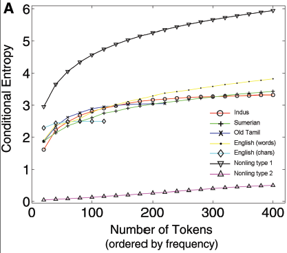
Rao et al. worked with a corpus of Indus Valley inscriptions, which recognizes 417 distinct symbol types. This is their "Indus" line. The other language lines come from different corpora in the indicated language. In each corpus, they filtered out the less common symbols, and then fit a first-order Markov chain. (Transition probabilities were estimated with a smoothing estimator rather than straight maximum likelihood.) Then they calculated the conditional entropy of the chain, using the estimated transition probabilities and the observed symbol frequencies (rather than say the invariant distribution of the chain); that's the vertical axis. The horizontal axis shows how many symbol types were retained --- i.e., "100 tokens" means that only the 100 most common symbols in the corpus were kept, and the chain was fit to those sequences. (This is not explained in the paper but was made clear in later correspondence between Sproat and the authors.) There are two lines for English, depending on whether "token" was taken to mean "character" (differentiating upper and lower case) or to mean "word".
The bottom curve shows the estimated conditional entropy from a purely deterministic sequence; the actual conditional entropy is in fact zero, so I presume that the upward trend is an artifact of the smoothed transition probabilities. The top curve, on the other hand, is from a uniform IID sequence --- here the real conditional entropy is the same as the marginal entropy, but both grow as N increases because the size of the symbol set grows. (I.e., this is an artifact of keeping only the most common symbols.)
Here is the flaw: there is no demonstration that only linguistic sequences have this pattern in their conditional entropies. Rao et al. have shown that two really extreme non-linguistic processes don't, but that's not a proof or even a plausibility argument. I would settle for an argument that non-linguistic processes have to be really weird to show this pattern, but even that is lacking. In Mayo's terms, they have not shown that this test has any severity.
Of course the fact that they haven't shown their test is severe doesn't mean that it isn't, in fact, severe. So, by way of procrastinating, I spent some time yesterday constructing a counter-example. My starting point was what Mark had done, generating a sequence of IID draws from a geometric distribution (rather than a uniform one) and subjecting it to the same analysis as Rao et al. As it happens, I had already written a function in R to fit Markov chains and calculate their log-likelihood, and here the conditional entropy is the negative log likelihood over the sequence length. (Admittedly this is only true using the maximum likelihood estimates for transition probabilities, rather than smoothed estimates as Rao et al. do, but my simulations had so much data this shouldn't matter.) Setting the rate of the geometric distribution to 0.075, here were my first results.
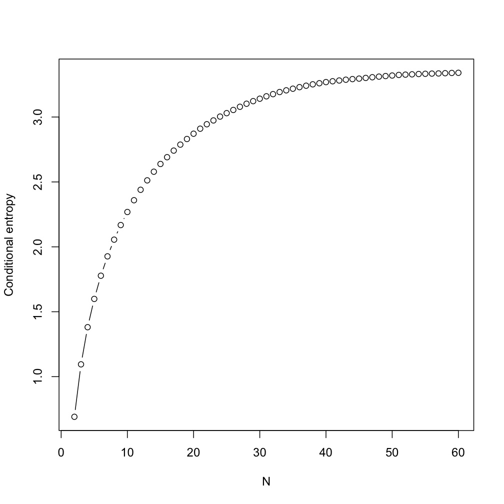
Mark Liberman and Richard Sproat did almost the same thing pretty much simultaneously, as you can see from the updates to Mark's post.
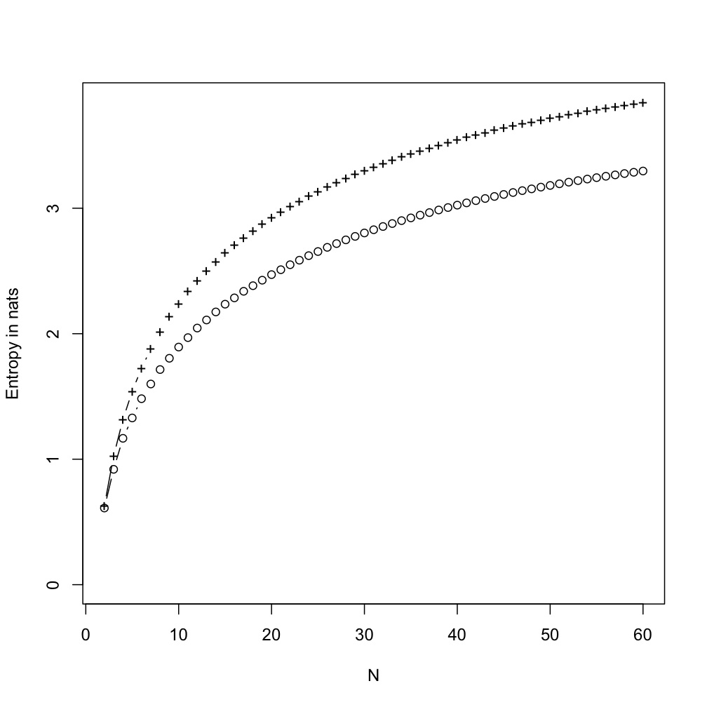
This was not entirely satisfactory, since (as Rao et al. point out in the online supplementary materials), there is a big gap between the marginal and conditional entropies for writing and for the Indus symbols. This was also, however, not too hard to finesse. In addition to the geometric sequence, I generated a Markov chain which alternated between the values +1 and -1, but where each positive or negative sign was 99% likely to be followed by the same sign. (That is, the signs were highly persistent.) I then multiplied the IID geometric variables (plus 1) by the Markov signs. This gave a larger set of symbols, but where knowing the sign of the current symbol (which "register" or "sub-vocabulary" it came from) was quite informative about the sign of the next symbol. (I added 1 to the geometric variables to exclude 0=-0, keeping the sub-vocabularies distinct.)
A third experiment takes after the fact that the Indus symbol sequences are all extremely short, at most a dozen characters or so. In stead of having a Markov chain for the sign, I used another, independent set of random draws, uniform on the integers from 2 to 6, to divide the sequence into blocks, and gave all the symbols in each block the same (coin-toss) sign.
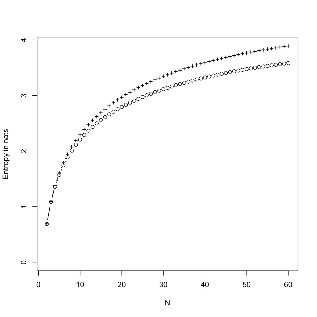
(Because I'm doing everything with a single long sequence, I artificially introduce transitions from positive to negative signs, which lowers the gap between the conditional and unconditional entropies. If I wanted to do this properly, I'd re-write my Markov estimator so it used many short sequences; but that would be too much like real work.)
The mechanism producing the gap between conditional and unconditional entropies is that the marginal distribution of symbols is a mixture of several pure distributions, and which mixture component we draw from now influences which component we'll draw from next (so the sequence can be Markov, exchangeable, etc.). Given the mixture components, the symbols are independent and the conditional and unconditional entropies are equal. Without that knowledge, the first symbol in effect is a cue for figuring out the mixture component, reducing the entropy of the second. There is nothing specifically linguistic about this; any hidden Markov model does as much. It would, for instance, work if the "symbols" were characters in randomly-selected comic books, who cluster (though slightly imperfectly); if that's too low-brow, think about Renaissance paintings, and the odds of seeing St. John the Baptist as opposed to a swan in one which contains Leda.
I have made no attempt to match the quantitative details Rao et al. report for the Indus symbols, just the qualitative patterns. Were I to set out seriously to do so, I'd get rid of the geometric distribution, and instead use a hidden Markov model with more than two states, each state having a distinct output alphabet, the distribution of which would be a Zipf (as used by Liberman or Sproat) or a Yule-Simon. (I might also try block-exchangeable sequences, as in my third example.) But this would approach real work, rather than a few hours of procrastination, and I think the point is made. Perhaps the specific results Rao et al. report can only be replicated by making distributional assumptions which are very implausible for anything except language, but I'd say that the burden of proof is on them. If, for instance, they analyzed lots of real-world non-linguistic symbol systems (like my comic books) and showed that all of them had very different conditional entropy curves than did actual writing, that would be a start.
I should in the interest of full disclosure say that a number of years ago Farmer and I corresponded about his work on the development of pre-modern cosmologies, which I find interesting and plausible (though very conjectural). But if anything I hope Farmer et al. are wrong and the Indus Valley civilization was literate, and I'd be extra pleased if the language were related to Tamil. Unfortunately, if that's the case it will need to be shown some other way, because these conditional entropy calculations have, so far as I can see, no relevance to the question at all.
My code (in R) is here if you want to play with this, or check if I'm doing something stupid. In the unlikely event you want more, I suggest reading the reply of Farmer et al., Rahul Siddharthan (especially the comments), or Fernando Pereira; the last is probably the wisest.
Manual trackback: Metadatta; Language Hat
Posted by crshalizi at April 28, 2009 22:30 | permanent link
Next week at the CMU statistics seminar, we give you all the Bayes you could want and more:
Posted by crshalizi at April 10, 2009 13:08 | permanent link
I will be completely offline from the 11th to 20th, while I contemplate whether certain referees deserve to be fed to jaguars, or whether it would not be more humane to sacrifice them to the great feathered serpent. (I mean humane to the cats, of course.)
Posted by crshalizi at April 10, 2009 13:00 | permanent link
Next week at the CMU statistics seminar:
Posted by crshalizi at April 03, 2009 13:37 | permanent link
Books to Read While the Algae Grow in Your Fur; Scientifiction and Fantastica; The Dismal Science; The Progressive Forces; The Continuing Crises; Writing for Antiquity; Cthulhiana
Posted by crshalizi at March 31, 2009 23:59 | permanent link
How many of the people currently pushing or exploiting conspiracy theories about the introduction of a global currency also claim to support returning to the gold standard?
(And where's Dan Sperber when we need him?)
The Dismal Science; The Running Dogs of Reaction; Psychoceramics
Posted by crshalizi at March 27, 2009 21:10 | permanent link
Attention conservation notice: Clearing out my drafts folder. 600+ words on some examples that I cut from a recent manuscript. Only of interest to (bored) statisticians.
The theme here is to construct some simple yet pointed examples where Bayesian inference goes wrong, though the data-generating processes are well-behaved, and the priors look harmless enough. In reality, however, there is no such thing as an prior without bias, and in these examples the bias is so strong that Bayesian learning reaches absurd conclusions.
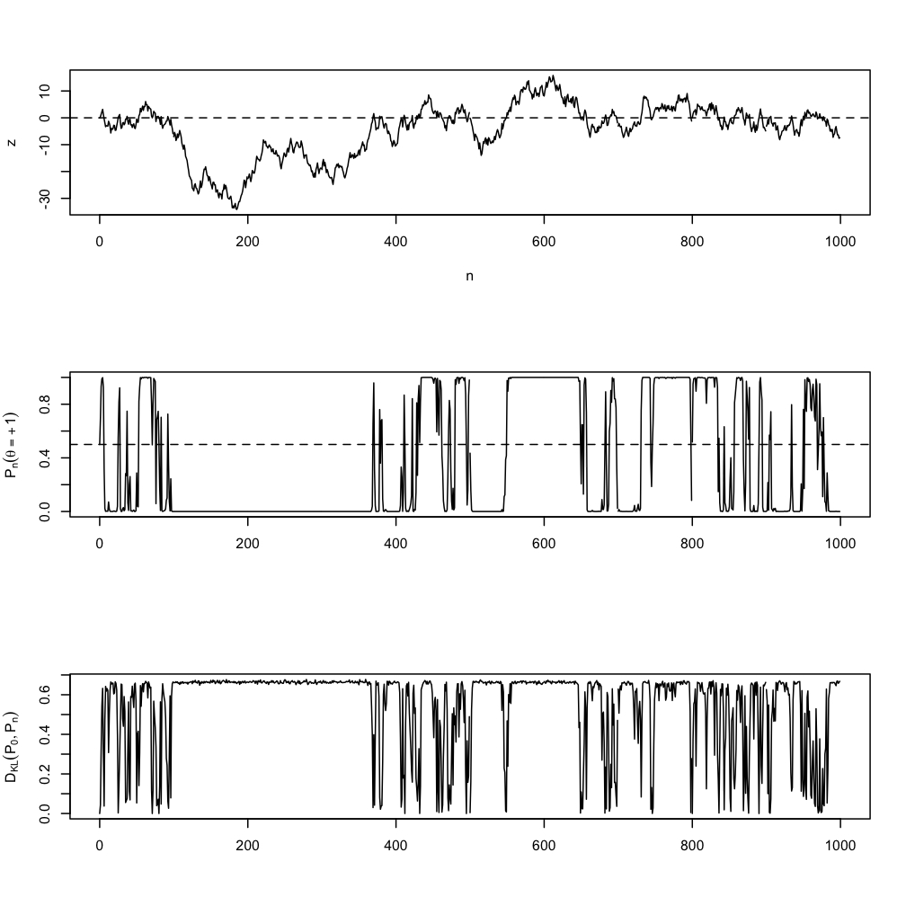
The data Xi, i=1,2,3,..., come from a 50/50 mixture of two Gaussians, with means at -1 and +1, both with standard deviation 1. (They are independent and identically distributed.) The prior, by coincidence, is a 50/50 mix of two Gaussians, located at -1 and +1, both with standard deviation 1. So initially the posterior predictive distribution coincides exactly with the actual data-generating distribution. After n observations x1, ... xn, whose sum is z, the log-likelihood ratio L(+1)/L(-1) is e2z. Hence the posterior probability that the expectation is +1 is 1/(1+e-2z), and the posterior probability that the expectation is -1 is 1/(1+e2z). The sufficient statistic z itself follows an unbiased random walk, meaning that as n grows it tends to get further and further away from the origin, with a typical size growing roughly like n1/2. It does keep returning to the origin, at intervals dictated by the arc sine law, but it spends more and more of its time very far away from it. The posterior estimate of the mean thus wanders from being close to +1 to being close to -1 and back erratically, hardly ever spending time near zero, even though (from the law of large numbers) the sample mean converges to zero.
This figure shows typical sample paths for z, for the posterior probability of the +1 mode, and for the relative entropy of the predictive distribution from the data-generating distribution. (The latter is calculated by Monte Carlo since I've forgotten how to integrate, so some of the fuzziness is MC noise.) Here is the R code.
Exercise 1: Confirm those calculations for the likelihood ratio and so for the posterior.
Exercise 2: Find the expected log-likelihood of an arbitrary-mean unit-variance Gaussian under this data-generating distribution.
Keep the same data-generating distribution, but now let the prior be the conjugate prior for a Gaussian, namely another Gaussian, centered at zero. The posterior is then another Gaussian, which is a function of the sample mean, since the latter is a sufficient statistic for the problem.
Exercise 3: Find the mean and variance of the posterior distribution as functions of the sample mean. (You could look them up, but that would be cheating.)
As we get more and more data, the sample mean of converges almost surely to zero (by the law of large numbers), which here drives the mean and variance of the posterior to zero almost surely as well. In other words, the Bayesian becomes dogmatically certain that the data are distributed according to a standard Gaussian with mean 0 and variance 1. This is so even though the sample variance almost surely converges to the true variance, which is 2. This Bayesian, then, is certain that the data are really not that variable, and any time now will start settling down.
Exercise 4: Suppose that we take the prior from the previous example, set it to 0 on the interval [-1,+1], and increase the prior everywhere else by a constant factor to keep it normalized. Show that the posterior density at every point except -1 and +1 will go to zero. (Hint: use exercise 2 and see here.)
Update in response to e-mails, 27 March: No, I'm not saying that actual Bayesian statisticians are this dumb. A sensible practitioner would, as Andy Gelman always recommends, run a posterior predictive check, and discover that his estimated model looks nothing at all like the data. But that sort of thing is completely outside the formal apparatus of Bayesian inference. What amuses me in these examples is that the formal machinery becomes so certain while being so wrong, while starting from the right answer (and this while Theorem 5 from my paper still applies!). See the second post by Brad DeLong, linked to below.
Manual trackback: Brad DeLong; and again Brad DeLong (with a simpler version of example 1!); The Statistical Mechanic
Posted by crshalizi at March 26, 2009 10:45 | permanent link
Attention conservation notice: back-of-the-envelope calculations about why the US has only about a fifth as many steelworkers now as it did in 1960. Not backed by any actual knowledge of the steel industry. Utterly untimely, it was, I think, prompted by a comment thread on Unfogged, but so long ago I can't remember which.
In 1960, US primary steel production was 91 million tons, of which 2.95 million tons were exported; it also imported 3.24 million tons. This part of the industry employed 530,000 people in all capacities, for an annual output of 170 tons/employee.
In 2007, US primary steel production was 98.1 million tons, with exports of 10.1 million tons and imports of 30.2 million tons. Employment was only 97,540 people, coming to 1005 tons/employee.
Exports and imports in 1960 were a wash, nearly enough, so let's suppose trade patterns had remained comparable and say that all of the net imports were to be made up by higher domestic production: (20.1 million tons)/(1005 tons/worker) = 20,000 extra workers. This would be a substantial increase, but it would still leave employment in steel at only 22% of its 1960 level. Where did the other four-fifths of the industry go?
The most obvious explanation is productivity. The industry in 2007 produced more than it did in 1960, with many fewer employees. In fact, output per employee grew 5.9 times over that period. A six-fold increase in productivity divided by a slight rise in total demand equals a roughly five-fold fall in employment.
Now, this calculation understates the effect of trade because it only considers net imports of steel. But steel is used as an input to producing many other things, and a washing machine made of steel shows up in this sort of official statistic as an import of a manufactured good, not an import of steel. So to really see what US steel production would be if we retained 1960 trade patterns, we'd need to see what the change in the (foreign*) steel content of US net imports has been. Since I don't have Leontief input-output matrices for the US and its trading partners in the two years, I can't do this.
Failing actual knowledge, I'll turn to guesswork. Suppose the steel content of imports was equal to net direct imports; this seems high, but what do I know? This would just add another 20,000 jobs, and bring us up to 26% of the size of the industry in 1960. To get the same level of employment in steel production now as in 1960, the net increase in the foreign steel content of our imports would have to satisfy
(530,000 workers) - (117,540 workers for domestic production and direct imports) = (increase in net indirect imports)/(1005 tons/worker)or 414,522,300 tons, i.e., about 3.5 times total production plus net direct imports. This is highly implausible.
I conclude that domestic employment in steel production has collapsed largely because increases in productivity have not been matched by increases in demand. If someone can point out where this reasoning goes wrong, I'd appreciate it.
*: Foreign steel content, because if the washing machine is made abroad of steel exported by the US, replacing that washing machine with a US-made one will not increase the demand for American steel.
Sources: 2007 employment figure from BLS (NAICS code 3311). 1960 employment figure from Table 1 on p. 2 of Lebergott. (It does not, however, appear to be affected by some of the well-known problems with Lebergott's series for the 1930s.) Annual production, import and export figures from USGS.
Manual trackback: The Inverse Square Blog; Nothing Funny About Feldspar (with more facts; go read)
Posted by crshalizi at March 24, 2009 10:49 | permanent link
O Hive Mind, o Lazy Web, Urania's child, I invoke thee! Is there a name
for the function
i.e., for when X is binomially distributed?
Posted by crshalizi at March 22, 2009 21:52 | permanent link
Exactly what bad consequences would follow if laws were passed by the relevant countries rendering credit default swap contracts void henceforth? (That is, canceling all the outstanding wagers because the bookies went bust.)
Update, 22 March: Well, one bad consequence would evidently be agreeing with Ben Stein. A bit from that link (by Felix Salmon, not Stein) is worth quoting:
There's a good chance, just for starters, that every major bank in America would go bust overnight: after all, they've been packaging up and selling off the credit risk on their multi-trillion-dollar loan portfolios [for years]. If Stein got his way, all that credit risk would suddenly reappear on the banks' balance sheets, and there's nothing they could do about it. Genius. Remember that those super-senior CDOs were the safest bits of the credit that they sold off. Just imagine what their balance sheets would look like if all the risky bits reappeared.
The issue he's raising is that if the banks can't say that they're covered for the risk of their loans defaulting (via the credit default swaps), they need to hold more capital as a protection against default. So as a legal or regulatory issue, ending the swaps would make the banks worse off. Substantively, however, this only makes sense if the swaps would, in fact, protect banks in the event of defaults — if they actually shifted the risk to the swap-sellers. Since we have just had pretty dramatic demonstrations that this is not something to be counted on, it's not at all clear to me that the banks ought to be able to keep that risk off their balance sheets. (In other words, the real value of the swaps to the banks is zero, or next to zero.) In any case, this objection could be countered by combining ending credit default swaps with public guarantees of the banks' existing positions — which is effectively what's happening anyway, only without making it harder to repeat the mistake in the future.
More broadly, ending credit default swaps would mean that those who sold such swaps would lose their stream of payments (a flow) but gain back their collateral and reserves (a stock); conversely buyers of default protection would gain a cash flow but take a hit to their capital stocks. Right now one imagines that even those selling the "end of the world trade" might prefer to get out of the game; I'd be interested to see an estimate of the effects of this on the stability of the financial world right now.
There is also the possibility that eliminating the swaps would deprive us of information about how risky different debts are. The value we should place on this, however, depends on how well these markets actually succeed in aggregating information about risk. I'd say there is abundant cause for skepticism about this — especially when things are, in fact, dangerous. Economic theory does not, in fact, provide any reason to think that such markets will be dominated by those with the most accurate beliefs (or even that the market as a whole will be more accurate than the best-informed trader), unless you assume a complete set of markets, which is a reductio ad absurdum if ever there were one. (When markets are incomplete, more markets are not necessarily better.)
To be clear, I am not asserting that credit default swaps should be ended. I honestly don't think I know enough to have an opinion about that, and while I'm obviously skeptical about their value, some serious and credible people (i.e., ones who do not have a vested interest in the matter) who've studied them in more depth see merit to them. If this is what a world with efficiently-allocated risk looks like, though, I'd hate to see a messed-up one.
(Thanks to readers D.H. and son1 for comments and pointers.)
Posted by crshalizi at March 17, 2009 22:22 | permanent link
Books to Read While the Algae Grow in Your Fur; Scientifiction and Fantastica; Complexity; The Dismal Science; Biology; The Progressive Forces; The Continuing Crises; Incestuous Amplification
Posted by crshalizi at February 28, 2009 23:59 | permanent link
My review of the book of Terence Tao's blog now out in the March-April 2009 issue of American Scientist. I wrote about Tao's blog a while ago, but there's a lot more in the review. Hopefully at least some of it is comprehensible.
— Having spent over fifteen years reading the magazine, especially for its book reviews, I am happy to finally have something printed there, but worry it means their standards are slipping.
Manual trackback: The Browser
Posted by crshalizi at February 14, 2009 22:48 | permanent link
Most networks support little or no trust. We will sometimes recognize segments of networks that qualify as trust-connected cliques. But the networks of drug use, blood distribution, and sexual contact through which HIV spreads, the networks through which routine political information flows, and the networks established by shared membership in voluntary associations mostly do not qualify. More generally, single-stranded networks containing few triads and sustaining little intimacy among their nodes rarely or never become trust networks.Characteristic enterprises in which trust networks figure importantly include cohabitation, procreation, provision for children, transmission of property, communication with supernatural forces, joint control of agricultural resources, long-distance trade, protection from [human] predators, maintenance of health, and collective response to disaster. With marked variation from setting to setting, trust networks often take the forms of religious sects and solidarities, lineages, trade diasporas, patron-client chains, credit networks, mutual aid societies, age grades, and local communities.
Books to Read While the Algae Grow in Your Fur; Scientifiction and Fantastica; The Progressive Forces; Networks; The Dismal Science; Enigmas of Chance; Writing for Antiquity; The Great Transformation; Food The Running Dogs of Reaction; The Beloved Republic
Posted by crshalizi at January 31, 2009 23:59 | permanent link
ALL YOUR BAYES ARE BELONG TO US |
we share with him |
Attention Conservation Notice: jargony, self-promotional ramblings about a new paper on the frequentist properties of non-parametric Bayesian procedures, which is exactly as statistics-geeky as it sounds. Plus a weird analogy to mathematical models of evolution. Even if this sounds vaguely interesting, you could always check back later and see if peer review exposed it as a tissue of fallacies.
Here's the new preprint:
There are people out there who see Bayes's Rule as the key to all methodologies, something essential to rationality. I find this view thoroughly misguided and not even a regulative ideal. But I've written about that at great length elsewhere and won't repeat myself here.
While there are certainly plenty of statisticians who embrace the Bayesian way in all its Savagery (some of them will be on my tenure committee), I think it's fair to say that most of the time, Bayesian methods are not used in contemporary statistics and machine learning to impose coherence on statisticians', or computers', personal beliefs. When people like Andy Gelman, Aleks Jakulin &c. estimate logistic regressions with a particular default prior, what they are doing is really regularization, which is something that a frequentist like me can understand.
Actually, Bayesian inference is a regularization-by-smoothing technique, only in the space of probability distributions instead of the sample space. In ordinary least-squares regression, one asks "what straight line comes closest (in the Euclidean sense) to all the data points?" In subtler methods, one has a whole menagerie of possible curves, and asks which superposition of curves comes closest to the data points. To avoid over-fitting, one needs to keep the weight given to very wiggly basis curves under control, e.g., by simply ignoring possible terms which are not sufficiently smooth. (Through the magic of Lagrange multipliers, this is equivalent to penalizing wiggliness.) As one gets more and more data, finer and finer features of the regression curve can be reliably discerned, so the amount of imposed smoothing should be relaxed. For estimating regression curves, this is all thoroughly understood and even automated (making the persistence of linear regression a mystery; but another time).
All of this carries over to estimating entire distributions rather than just curves. In the space of probability distributions, the entire sample is a single point, the empirical distribution. (I'm ignoring some subtleties about time series here.) The family of models we're willing to consider forms a manifold (or set of manifolds; more details) in the space of probability measures. In this space, the right way to measure distance isn't the Euclidean metric, but rather the relative entropy, a.k.a. the Kullback-Leibler divergence, which generates the information geometry. The maximum likelihood estimate is simply the geometric projection of the empirical distribution on to the manifold of models. In other words, the most likely predictive distribution comes from this single point on the manifold. (There are cleverer ways to get frequentist predictive distributions, though.) The Bayesian posterior predictive distribution gives some weight to all points on the manifold; this is the smoothing. The weights are proportional to the prior, and also decline exponentially with the product of sample size and relative entropy. The effect of the prior is to blunt the impact of what we actually see, keeping us from simply trying to match it — exactly like the effect of smoothing. The amount of smoothing done by the prior declines as the sample size grows.
Why smooth or regularize in the first place? As every school-child knows, the answer lies in the bias-variance trade-off. (Pedantically, bias-variance is for mean-squared error, but other loss functions have similar decompositions.) Regularized estimates are less responsive to differences between data sets, which means that they have less variance. No matter what the data look like, the regularized estimates all have the same shape, so to speak. But unless reality also has that shape, this creates a systematic error, i.e., bias. So the more aggressively we smooth, the more we decrease variance, but the more we increase bias. If some degree of smoothing removes more variance than it adds bias, we come out ahead. Of course, the variance should fall automatically as we get more data, but the bias depends on the strength of smoothing, so the latter should shrink as the sample grows. The important thing in analyzing this type of estimation or prediction scheme is to check whether they relax their regularization at the right rate, so that they don't get killed by either bias or variance, but rather consistently converge on the truth, or at least the best approximation to the truth among the available models.
All of this applies to Bayesian learning. Like any other regularization scheme, it is a way of deliberately introducing bias into our inferences, not so much on Burkean/Quinean grounds that our prejudices providentially point to the truth, but simply to reduce variance, the extent to which our inferences are at the mercy of Fortune (in her role as the goddess of sampling fluctuations). The question about it then becomes whether it gets the trade-off right, and manages to converge despite its bias. In other words, when does Bayesian inference possess frequentist consistency?
A surprisingly large number of people have been satisfied with a result given by the great probabilist J. L. Doob, which essentially says that under some reasonable-looking conditions, the Bayesian learner's prior probability of being inconsistent is zero. (More exactly, the posterior probability of any set of models containing the truth goes to 1, except on a set of sample paths whose prior probability is zero.) Even taken at face value, this just says that each Bayesian is convinced a priori that they'll converge on the truth, not that they actually are almost sure to find the truth.
Examining the reasonable-looking conditions of Doob's result, it turns out that they entail the existence of a consistent non-Bayesian estimator. (Doob's original assumptions can actually be weakened to just the existence of such an estimator; see Schervish's Theory of Statistics, ch. 7.) It is a curious fact that every proof of the consistency of Bayesian learning I know of requires the existence of a consistent non-Bayesian estimator. (Though it need not be the maximum likelihood estimator.) There don't seem to be any situations where Bayesian updating is the only convergent route to the truth.
It turns out that Bayesian inference is not consistent in general. The late David Freedman and the very-much-alive Persi Diaconis showed that if you choose a prior distribution which is badly adapted to the actual data-generating process, your posterior distribution will happily converge on the wrong model, even though the rest of the set-up is very tame — independent and identically distributed data in a boringly well-behaved sample space, etc.
Still, there are many situations where Bayesian learning does seem to work reasonably effectively, which in light of the Freedman-Diaconis results needs explaining, ideally in a way which gives some guidance as to when we can expect it to work. This is the origin of the micro-field of Bayesian consistency or Bayesian nonparametrics, and it's here that I find I've written a paper, rather to my surprise.
I never intended to work on this. In the spring of 2003, I was going to the statistics seminar in Ann Arbor, and one week the speaker happened to be Yoav Freund, talking about this paper (I think) on model averaging for classifiers. I got hung up on why the weights of different models went down exponentially with the number of errors they'd made. It occurred to me that this was what would happen in a very large genetic algorithm, if a solution's fitness was inversely proportional to the number of errors it made, and there was no mutation or cross-over. The model-averaged prediction would just be voting over the population. This made me feel better about why model averaging was working, because using a genetic algorithm to evolve classifier rules was something I was already pretty familiar with.
The next day it struck me that this story would work just as well for Bayesian model averaging, with weights depending on the likelihood rather than the number of errors. In fact, I realized, Bayes's rule just is the discrete-time replicator equation, with different hypotheses being so many different replicators, and the fitness function being the conditional likelihood.
As you know, Bob, the replicator dynamic is a mathematical representation of the basic idea of natural selection. There are different kinds of things, the kinds being called "replicators", because things of one kind cause more things of that same kind to come into being. The average number of descendants per individual is the replicator's fitness; this can depend not only on the properties of the replicator and on time and chance, but also on the distribution of replicators in the population; in that case the fitness is "frequency dependent". In its basic form, fitness-proportional selection is the only evolutionary mechanism: no sampling, no mutation, no cross-over, and of course no sex. The result is that replicators with above-average fitness increase their share of the population, while replicators with below-average fitness dwindle.
This is a pretty natural way of modeling half of the mechanism Darwin and Wallace realized was behind evolution, the "selective retention" part — what it leaves out is "blind variation". Even with this omission, the replicator equation is a surprisingly interesting kind of dynamical system, especially when fitness is frequency-dependent, which opens up deep connections to evolutionary game theory. (ObBook.) Interestingly, however, Bayes is a very limited special case of the replicator equation, since fitness is frequency independent.
"Selective retention" is also the idea that lies behind reinforcement learning and Thorndike's law of effect. Crudely, these are all variations on the theme of "do more of what worked, and less of what didn't". Less crudely, there are at least three independent discoveries of how reinforcement learning, itself, leads to the replicator equation in the appropriate limit. So Bayesian updating isn't just a special case of evolutionary optimization; it's also something like habit formation.
Initially, I wrote this all up in the spring of 2003 and then set it aside, because, after making the formal connections, I didn't see what it was good for. Then, that summer, I went to the first "Science et Gastronomie" workshop, talked about this idea, and realized, from the conversations, that I actually could do something with it. The fitness function was going to end up being the relative entropy rate, and this would control where the posterior distribution concentrated in the long run. This would let me say something about the convergence of Bayesian learning with non-independent and even non-Markovian data, but also about what happens when the true distribution is not "in the support of the prior", i.e., when all the models really are wrong.
So I spent a lot of time in Lyon sweating over the asymptotic behavior of the integrated likelihood and so forth (literally, given the great heat-wave). By the end of the summer, I had versions of what are now Theorems 2, 3 and 4 in the paper. These say, respectively, that the posterior density goes to zero everywhere where fitness isn't maximized, and the rate is the fitness difference; that eventually the posterior distribution concentrates on the global peaks of the fitness landscape; and that the posterior distribution in a subset of model space not including those peaks is driven by the highest fitness in the subset. All of this was pretty nice and I was fairly pleased with myself.
Then I saw that if my results were correct, Bayesian updating should always be consistent. So I put the thing aside for a while....
Eventually I figured out what I was doing wrong; I was presuming that all the points in model-space were equally well-behaved. I was explicitly assuming that the (log) likelihood would eventually converge to the relative entropy for each hypothesis. This is on the one hand mathematically harmless (it's asymptotic equipartition), and on the other hand statistically I can't see how any likelihood-based method can hope to converge unless performance over a sufficiently long past is indicative of future results. (This is why such methods do not solve the problem of induction.) But I was further assuming, implicitly, that there was no way for the likelihood of a hypothesis with very high relative entropy to also converge very slowly. That is, I was assuming the Bayesian learner could not acquire bad habits. But of course it can; the bad habits just need to seem like good ideas at first. In human terms:
No one ever forgets how to do something that's worked for them in the past. Just replacing it with another behavior can be hard enough, and the old behavior is still going to be lurking there underneath it. Thieves keep stealing. Liars keep lying. Drunks never forget about chemically modifying their nervous systems.Similarly, the Bayesian learner never forgets about the model which matches the data perfectly — until it turns out that the model had just memorized the first 13,127 observations, and then repeats them forever. When that model crashes, however, there is always another one which memorized the first 26,254 observations...
What's needed is some restrictions on the prior distribution which keep it from putting too much weight on these bad hypotheses, though actually in non-parametric problems one doesn't want to give them strictly zero weight, because, hey, maybe a particular sequence of 13,127 observations really will repeat forever. (Metaphorically: a little lying, stealing and drinking is part of a complete life.) We are back to regularization, which has the duty of promoting virtue and suppressing vice.
The most common ways of doing this divide the space of models into distinct classes, and then use statistical learning theory or empirical process theory to gauge the risk of over-fitting within these constrained subspace. Typical arguments involve things like showing that every hypothesis in the constrained set is close to one of a finite number of hypotheses which "cover" or "bracket" the space, which gives uniform convergence. Then one relaxes the constraint as more data arrives, according to some deterministic schedule ("the method of sieves") or to optimize the trade-off between actual performance and a bound on over-fitting ("structural risk minimization"), etc.
Existing proofs of Bayesian consistency in non-parametric problems basically work similarly. To simplify just a bit, the trick has two parts. The first is to find constraints on the hypotheses which are strong enough to ensure uniform convergence, but can be relaxed to include everything; this is what you'd do anyway if you wanted a consistent non-parametric procedure. (Some people don't explicitly posit constraint sets, but do other things with much the same effect.) The second is to construct a prior whose bias towards the most-constrained sets is strong enough to keep the wild, high-capacity parts of the hypothesis space from dominating the posterior distribution, but isn't so biased that the constraint can't be overcome with enough data.
This is what I ended up having to do. (There was a gap of several years between seeing that some constraint was needed, and seeing what constraint would work. I am, in fact, a sloth.) My constraint was, roughly, "the log likelihood converges at least this fast". Unfortunately, I wasn't able to express it in relatively nice terms, like covering numbers, though I suspect someone cleverer could replace it with something along those lines. (It's about one-sided deviations of time-averages from their limiting values, so it feels empirical-process-y.) Anyone who actually cares will actually be better served by reading the paper than by my trying to re-express it verbally.
I didn't figure out the right constraint to impose, and the right way to relax it, until the summer of 2008. (This was what was on my mind when I read Chris Anderson's ode to overfitting.) Once I did, everything else was pretty direct, especially since it turned out I could salvage most (but definitely not all) of what I'd done in Lyon. One of the bigger efforts in actually writing the paper was uniformly eliminating talk of replicators and fitness, except for a small appendix, in favor of more statistical jargon. (I hope I succeeded.) Adding an example, namely trying to use Markov chains to predict a sofic system, took about a day. This is an amusing case, because the posterior distribution never converges — you can always do strictly better by moving to Markov chains of higher order. Nonetheless, the (Hellinger) distance between the posterior predictive distribution and the actual predictive distribution goes to zero.
Having submitted this, I'm going to put it aside again until I hear from the referees, because there's a lot of other work which needs finishing. (When I do hear from the referees, I anticipate a certain amount of gnashing of teeth.) But in the meanwhile, I'll use this space to jot down some ideas.
Manual Trackback: 3 Quarks Daily
Thanks to Nicolas Della Penna, Shiva Kaul and Chris Wiggins for typo-spotting.
Posted by crshalizi at January 30, 2009 22:47 | permanent link
Restoring stolen goods to their rightful owners is not Pareto-improving.
Posted by crshalizi at January 29, 2009 09:08 | permanent link
Now would be an excellent time to begin working like we are living in the early days of a better nation.
Let those who do justice and love mercy say amen.
Posted by crshalizi at January 20, 2009 23:11 | permanent link
If, even a month ago, you had asked me who I'd most like to see elected to Congress, I would not have mentioned Tom Geoghegan, because it wouldn't have even occurred to me that it was possible. Had you asked me about him in particular, I would have replied something on the order of "We should be so lucky". But he's running in the special election to replace Rahm Emanuel, and, well, we the people should be so lucky. The estimable Kathy G. has explained why Geoghegan deserves the support of progressives everywhere. I have nothing to add, other than to say that (1) if you haven't read Which Side Are You On?, you should buy it right now and read it at once; and (2) I have just put my money where my mouth is.
Posted by crshalizi at January 10, 2009 21:45 | permanent link
Attention conservation notice: ~500 words of excessively cute foundations-of-statistical-mechanics geekery. Inspired by this post at The Statistical Mechanic.
I have here on the table before me my favorite classical-mechanical assemblage of interacting particles, with 2n degrees of freedom, n being a macroscopically large number. (The factor of 2 is both because there are always position and velocity degrees of freedom, and to avoid some factors of 1/2 later.) It is in turn part of a larger assemblage with many more degrees of freedom, say 2N. Both the smaller and larger assemblages are highly unstable dynamically, so I can expect statistical mechanics to work quite well. (Really, I can.) On the other hand, I presume that they are very thoroughly isolated from the rest of the universe, so I can ignore interactions with the outside. (Don't ask me how I know what's going on in there in that case, though.)
I have also an Aberdeen Mfg. Mk. II "Neat-fingered" Maxwellian demon, which is capable of instantaneously reversing all the velocities of the particles in the small assemblage (i.e., it can flip the sign of n velocity degrees of freedom). If I had a bigger research budget, I could have bought a Mk. V "Vast and Considerable" demon, which could reverse the whole assemblage's N velocity degrees of freedom, but I don't have to tell you about grants these days.
Now, with the Mk. V, I'd know what to expect: it's the old familiar myth about time's arrow running backwards: sugar spontaneously crystallizing out of sweetened coffee, forming granules and leaping out of the cup into the tea-spoon, etc. But the Mk. II isn't capable of reversing the arrow of time for the whole assemblage, just for part of it. And so there are N-n degrees of freedom in the larger assemblage whose arrow of time points the same way as before. So what happens?
My intuition is that at first the arrow of time is reserved in the small assemblage, leading to the local equivalent of coffee unsweetening. ("At first" according to who? Don't go there.) Eventually, however, interactions with the N-n unreversed degrees of freedom should bring the n degrees of freedom back into line. If interactions are spatially local, then I imagine the time-reversed region gradually shrinking. Mythologically: The sugar crystallizes and forms granules, say, and even starts to leap out of the cup, but neither the air molecules nor the spoon are in the right place at the right time to exactly take them back to sugar-jar, so they spill and make a mess, etc. More generally, an observer within the larger assemblage will first see a small region where, bizarrely, things happen in reverse, then a kind of hard-to-describe crawling molecular chaos, and then a restoration of the ordinary macroscopic natural order, albeit from a weird starting point. But this guess may be excessively shaped by the fluctuation-dissipation theorem. Does a single arrow of time have to get established at all? If so, how long does it typically take? (Intuition again, this time from large deviations: exponential in 2n-N.) Can the n reversed degrees of freedom ever impose their direction on the whole assemblage?
Somebody must have already looked into all this. Where?
Update, later that afternoon: I was probably unconsciously remembering this post by Sean Carroll. (Sean was very polite in pointing this out.) Also, John Burke answers my final "where" question "Budapest", which sounds about right.
Posted by crshalizi at January 10, 2009 13:45 | permanent link
I will be teaching 36-462, "topics in statistics", in the spring. This is a special topics course for advanced undergraduates, intended to expose them ideas they wouldn't see going through the ordinary curriculum; this year, like last, the subject will be "chaos, complexity and inference". It worked pretty well last time, though I am not sure what to make of the fact that half of those currently registered are graduate students from other departments...
Anyone interested in the readings, assignments and notes can follow them either at the class syllabus page, or from this post and its RSS feed. (Last year's post.) — There have been some requests (as in, more than one!) for podcasts of the lectures. If someone will point me at an idiot's guide to setting one up, and tell me about cheap but adequate microphones, I'm willing to try.
Posted by crshalizi at January 08, 2009 23:59 | permanent link